Throughout my professional journey, I’ve encountered numerous situations requiring me to craft intricate analytical queries for various reports and visualizations. Frequently, these involved charts that presented data aggregated by time periods like date, week, or quarter. Such reports are typically generated to assist clients in spotting patterns and understanding their business performance from a broader perspective. However, challenges arise when data scientists and engineers need to create far more comprehensive reports based on massive datasets.
For reports based on smaller datasets, a simple SQL query executed against a relational database can suffice. It’s crucial to have a solid grasp of query writing fundamentals and optimization techniques to ensure efficiency. Yet, when dealing with substantially larger datasets (e.g., millions or even billions of rows) and the reports don’t rely heavily on dynamic input parameters or have a limited set of parameter values, SQL queries can become sluggish. Making users wait for such queries to complete is far from ideal. The prevalent practice in these scenarios is to pre-run the queries before clients request the reports.
This approach often involves implementing some form of caching mechanism, enabling the client to retrieve data from the cache instead of triggering real-time query execution. While effective, this method is most suitable when real-time data is not a necessity, as the displayed data might be calculated with a delay, ranging from an hour to even a day. Consequently, the reports and charts utilize cached data rather than reflecting real-time information.
Leveraging Google BigQuery
During my involvement in an analytical project within the pharmaceutical sector, I encountered a requirement for charts that accepted zip code and drug name as input parameters. Additionally, the charts needed to showcase comparisons between drugs across specific US regions.
The analytical query underpinning these charts proved to be highly complex, taking approximately 50 minutes to execute on our Postgres server (equipped with a quad-core CPU and 16 GB of RAM). Pre-running and caching the results was impractical due to the dynamic nature of the input parameters (zip codes and drugs), resulting in thousands of potential combinations that made prediction impossible.
Even attempting to execute all parameter combinations would have likely overwhelmed our database. This situation necessitated exploring alternative approaches and seeking a more manageable solution. The client, while valuing the importance of the chart, was hesitant to commit to substantial architectural changes or a complete database migration.
We experimented with a few different strategies during this project:
- Scaling the Postgres server vertically by augmenting its RAM and CPU resources.
- Evaluating alternative database solutions such as Amazon Redshift and others.
- Investigating NoSQL options, though most of them introduced significant complexity and demanded extensive architectural modifications, which the client was unwilling to undertake.
Ultimately, we turned to Google BigQuery. It fulfilled our requirements and enabled us to deliver the desired functionality without necessitating major changes that might have been met with resistance from the client. But what exactly is Google BigQuery, and what accounts for its efficacy?
BigQuery is a REST-based web service designed for executing sophisticated SQL-like analytical queries against massive datasets. Upon uploading our data to BigQuery and running the same query that had previously taken 50 minutes on our Postgres server (with a remarkably similar syntax), we witnessed a remarkable reduction in execution time to around one minute. This translated to an impressive 50x performance improvement simply by adopting a different service. It’s worth highlighting that other database solutions we explored fell significantly short of delivering comparable performance gains. Honestly, the performance boost achieved with BigQuery was genuinely remarkable, surpassing even our most optimistic expectations.
However, it’s important to acknowledge that BigQuery, despite its strengths, is not a one-size-fits-all database solution. While highly effective for our particular use case, it comes with certain limitations, such as restrictions on the number of daily table updates, data size limits per request, and more. It’s crucial to understand that BigQuery is not intended as a direct replacement for a relational database; its focus lies in handling analytical queries, not basic CRUD (Create, Read, Update, Delete) operations or simpler queries.
In this article, I aim to provide a comparative analysis of Postgres (my preferred relational database) and BigQuery in the context of real-world scenarios. Additionally, I’ll offer some recommendations on when it’s genuinely advantageous to leverage BigQuery.
Sample Data
To facilitate a meaningful comparison between Postgres and Google BigQuery, I utilized publicly available demographic data for various countries. This data was grouped by country, age, year, and sex (you can obtain the same dataset from this link).
I structured the data into four tables:
populationslocationsage_groupspopulations_aggregated
The final table, populations_aggregated, contains pre-aggregated data derived from the first three tables. Below is the database schema:
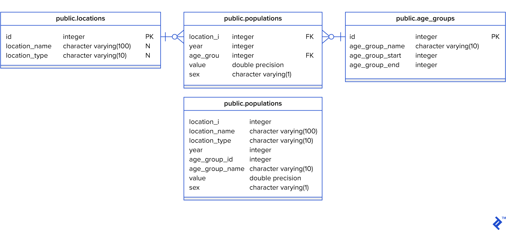
The populations table I worked with contained over 6.9 million rows—not an exceptionally large dataset, but sufficient for my testing purposes.
Using this sample data, I crafted queries designed to resemble those used for generating real-world analytical reports and visualizations. The queries were aimed at answering the following questions:
- What is the population of the US aggregated by year?
- What is the population of all countries in 2019, sorted in descending order starting with the most populous?
- Which are the top five “oldest” nations for each year? “Oldest” in this context refers to countries with the highest percentage of their population aged 60 and above. The query should return five results per year.
- Which are the top five nations for each year with the most significant difference between their male and female populations?
- What is the median age per country for each year, sorted from the “oldest” to the “youngest” countries?
- Which are the top five “dying” countries for each year? “Dying” signifies countries experiencing the most substantial population decline.
Queries #1, #2, and #6 are relatively straightforward. However, queries #3, #4, and #5 posed a greater challenge to formulate, at least from my perspective. It’s important to note that I primarily identify as a back-end engineer, and writing complex SQL queries isn’t my forte. Individuals with more specialized SQL expertise could likely devise more optimized queries. Nonetheless, our objective is to compare how Postgres and BigQuery handle the same queries against the same dataset.
In total, I constructed 24 queries:
- 6 queries targeting the non-aggregated tables (
populations,locations,age_groups) in the Postgres database. - 6 queries targeting the
populations_aggregatedtable in the Postgres database. - 6 queries targeting the non-aggregated tables in BigQuery.
- 6 queries targeting the aggregated table in BigQuery.
To illustrate, let’s examine BigQuery queries #1 and #5 for the aggregated data, providing a glimpse into the complexity of a simple query (#1) and a more intricate one (#5).
Population in the US aggregated by year query:
| |
Query for median age per country per year, sorted from oldest to youngest:
| |
Note: You can access all the queries in my Bitbucket repository (link provided at the end of the article).
Test Results
I used two distinct Postgres servers to execute the queries. The first server had 1 CPU core, 4 GB of RAM, and was backed by an SSD drive. The second server was considerably more powerful, boasting 16 CPU cores, 64 GB of RAM, and also utilizing an SSD drive. Essentially, the second server had 16 times the CPU and RAM capacity of the first.
It’s crucial to highlight that the databases were idle during the test, meaning no other queries were contending for resources. In real-world scenarios, query execution times would likely be longer due to concurrent queries potentially introducing contention and table locks. I used pgAdmin3 and the BigQuery web interface to measure query execution speeds.
The test yielded the following results:
| Postgres (1 CPU 4 RAM, SSD) | Postgres (16 CPU 64 RAM, SSD) | BigQuery | ||||
| Aggregated | Non-aggregated | Aggregated | Non-aggregated | Aggregated | Non-aggregated | |
| Query 1 (US Population aggregated by Years) | 1.3s | 0.96s | 0.87s | 0.81s | 2.8s | 2.4s |
| Query 2 (Population by Countries in 2019) | 1.1s | 0.88s | 0.87s | 0.78s | 1.7s | 2.6s |
| Query 3 (Top 5 Oldest nations by years) | 34.9s | 35.6s | 30.8s | 31.4s | 15.6s | 17.2s |
| Query 4 (Top 5 Countries with the biggest difference in male and female population) | 16.2s | 15.6s | 14.8s | 14.5s | 4.3s | 4.6s |
| Query 5 (Age median per country, year) | 45.6s | 45.1s | 38.8s | 40.8s | 15.4s | 18s |
| Query 6 (Top 5 "Dying" countries per year) | 3.3s | 4.0s | 3.0s | 3.3s | 4.6s | 6.5s |
Let’s visualize these results using bar charts for query #1 and query #5:
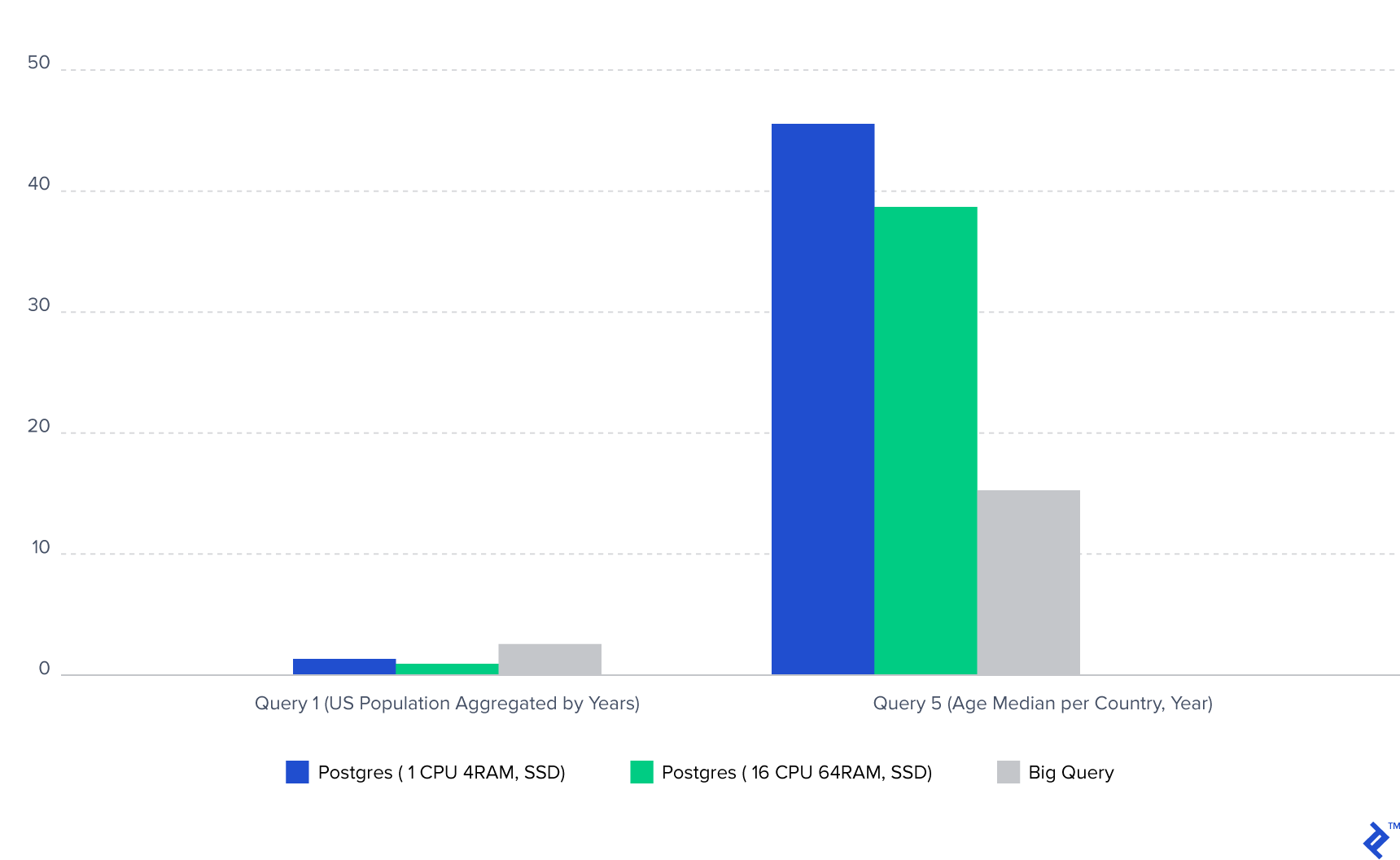
Note: The Postgres database was hosted on a US-based server, while I’m located in Europe, introducing network latency that contributed to the overall execution time for Postgres.
BigQuery Performance and Insights
Based on the test results, several key observations emerged:
- Vertically scaling Postgres, even by a factor of 16, only yielded a performance improvement of 10-25% for single-query execution. In essence, the Postgres server with a single CPU core and 4 GB of RAM exhibited query execution times comparable to those of the server with 16 CPU cores and 64 GB of RAM. While larger servers can accommodate significantly larger datasets, they don’t necessarily translate to substantial reductions in individual query execution time.
- In Postgres, joins involving small tables (the
locationstable had around 400 rows, and theage_groupstable had 100 rows) didn’t result in significant performance differences compared to queries against the aggregated data residing in a single table. Moreover, I observed that for queries completing within a few seconds, those utilizing inner joins were generally faster. However, for longer-running queries, this pattern didn’t always hold true. - BigQuery exhibited a contrasting behavior regarding joins. It exhibited a notable aversion to joins, as evidenced by the substantial time discrepancies between queries operating on aggregated data versus those querying non-aggregated data (for queries #3 and #5, the difference was around two seconds). This suggests that while BigQuery can accommodate numerous subqueries, achieving optimal performance often necessitates querying a single table.
- Postgres consistently outperformed BigQuery for queries involving simple aggregations, filtering, or smaller datasets. Specifically, I found that queries completing within five seconds in Postgres generally took longer to execute in BigQuery.
- BigQuery truly shone when handling long-running queries. As the size of the dataset grew, the performance gap between Postgres and BigQuery widened considerably.
When to Consider Google BigQuery
Let’s circle back to the central question: when is it appropriate to utilize Google BigQuery? Based on the insights gained, I’d recommend considering BigQuery when the following conditions are met:
- You frequently encounter queries that take more than five seconds to execute against your relational database. BigQuery’s strength lies in processing complex analytical queries, making it less suitable for simpler queries involving basic aggregations or filtering. It excels when dealing with “heavy” queries that operate on large datasets. The larger the dataset, the more pronounced the performance benefits of using BigQuery are likely to be. Recall that the dataset I used was only 330 MB.
- BigQuery’s performance is hampered by joins, so consolidating your data into a single table is advisable to achieve faster execution times. BigQuery allows you to persist query results into new tables. Therefore, to create an aggregated table, you can upload all your data to BigQuery, execute a query that aggregates the data as needed, and save the results into a new table.
- BigQuery’s built-in caching mechanism makes it well-suited for scenarios where data doesn’t change frequently. This means that if you run the same query multiple times and the underlying data in the tables remains unchanged, BigQuery will serve the results from its cache, eliminating the need to re-execute the query. Importantly, BigQuery doesn’t incur charges for cached queries. However, it’s worth noting that even cached queries might take 1-1.2 seconds to return results.
- Offloading analytical queries to BigQuery can be an effective strategy for reducing the load on your primary relational database. Analytical queries are resource-intensive, and excessive reliance on them within a relational database can lead to performance bottlenecks, potentially forcing you to contemplate scaling your database server. By migrating these queries to BigQuery, you alleviate the burden on your core relational database.
In conclusion, a few more points are worth mentioning regarding BigQuery’s real-world usage. In our project, the report data was refreshed on a weekly or monthly basis, allowing for manual data uploads to BigQuery. However, if your data changes frequently, synchronizing data between your relational database and BigQuery can become more intricate and is something to factor into your decision-making process.
Links
You can access the sample data used in this article by following this here, while the queries and data in CSV format are available at here.