Throughout history, computational science has primarily been the domain of researchers and PhD students. However, what the broader software development community might not realize is that us scientific computing enthusiasts have been diligently building collaborative, open-source libraries that do most of the hard work. Consequently, implementing mathematical models is now simpler than ever. Although the field might not be ready for widespread use yet, the barrier to entry has significantly decreased. Creating a new computational codebase from scratch is a massive task, often taking years, but these open-source scientific computing projects, with their accessible examples, allow for relatively quick utilization of these capabilities.

Scientific computing aims to provide insights into real-world systems, pushing the boundaries of how software can represent reality. Accurately simulating the real world with high fidelity requires intricate differential mathematics, knowledge typically confined to universities, national labs, or corporate R&D departments. Moreover, expressing the continuous, infinitesimal nature of reality using the discrete language of computers presents significant numerical hurdles. It demands a meticulous transformation process to create algorithms that are both computationally manageable and yield meaningful outcomes. In short, scientific computing is no easy feat.

Open Source Tools for Scientific Computing

I have a personal affinity for the FEniCS project, having used it for my thesis. Therefore, it will be the foundation for our code example in this tutorial. (Note that other excellent projects like DUNE exist and can be used as well.)

FEniCS describes itself as “a collaborative project developing innovative concepts and tools for automated scientific computing, particularly focused on automating the solution of differential equations using finite element methods.” This powerful library tackles a wide array of problems and scientific computing applications. Contributors from institutions like Simula Research Laboratory, the University of Cambridge, the University of Chicago, Baylor University, and KTH Royal Institute of Technology have collectively built it into an invaluable resource over the past decade (see the FEniCS codeswarm).

The sheer amount of effort the FEniCS library spares us is remarkable. To grasp the impressive depth and breadth of topics it covers, one can view their open source text book. Notably, Chapter 21 even compares various finite element schemes for solving incompressible flows.

Behind the scenes, the project integrates a vast collection of open-source scientific computing libraries, which may be of interest or use directly. These include, in no particular order:

• PETSc: Tools for the scalable solution of scientific applications modeled by partial differential equations.
• Trilinos Project: Reliable algorithms for solving linear and non-linear equations, stemming from work at Sandia National Labs.
• uBLAS: A C++ template class library offering fundamental linear algebra functionality and algorithms.
• GMP: A library for arbitrary precision arithmetic, handling various numerical data types.
• UMFPACK: Routines for solving unsymmetric sparse linear systems using the Unsymmetric MultiFrontal method.
• ParMETIS: An MPI-based library for partitioning graphs and matrices and computing orderings for sparse matrices.
• NumPy: The core package for scientific computing with Python.
• CGAL: A C++ library providing robust and efficient algorithms for geometric computations.
• SCOTCH: Software for graph and mesh partitioning, mapping, clustering, and sparse matrix ordering.
• MPI: A widely used standard for message-passing in parallel computing environments.
• VTK: A comprehensive system for 3D computer graphics, image processing, and visualization.
• SLEPc: A library designed for solving large-scale eigenvalue problems on parallel computers.

This list of integrated external packages hints at the capabilities FEniCS inherits. For instance, MPI support enables scaling across multiple machines in a compute cluster (meaning the code can run on a supercomputer or your laptop).

Interestingly, these projects have potential applications beyond scientific computing, such as financial modeling, image processing, optimization problems, and even video game development. Imagine a video game that leverages these open-source algorithms to simulate two-dimensional fluid flow, like ocean currents, for players to interact with (perhaps sailing a boat through varying wind and water conditions).

A Sample Application: Using Open Source for Scientific Computing

This section demonstrates how a basic Computational Fluid Dynamics scheme is developed and implemented using one of these open-source libraries—specifically, the FEniCS project. FEniCS offers APIs in Python and C++. This example utilizes their Python API.

We will delve into some technical details. However, the goal is simply to provide a glimpse into developing such scientific computing code and showcase how much easier today’s open-source tools make it. Hopefully, this will help demystify the often-perceived complex world of scientific computing. (An Appendix provides detailed mathematical and scientific explanations for those interested.)

DISCLAIMER: Readers unfamiliar with scientific computing software may find parts of this example challenging:

Don’t worry if that’s the case. The key takeaway is how existing open-source projects can drastically simplify many of these tasks.

With that in mind, let’s examine the FEnICS demo for incompressible Navier-Stokes. This demo models the pressure and velocity of an incompressible fluid moving through an L-shaped bend, like a plumbing pipe.

The description on the linked demo page provides an excellent, concise explanation of the steps involved in running the code. I encourage you to take a look to see what’s involved. Briefly, the demo simulates the fluid flow over time, animating the results. It achieves this by setting up a mesh representing the space within the pipe and using the Finite Element Method to numerically solve for the velocity and pressure at each point on the mesh. The simulation proceeds iteratively, updating the velocity and pressure fields over time using the equations at hand.

The demo works well as is, but we’ll make a slight modification. While it utilizes the Chorin split, we’ll implement the slightly different Kim and Moin method, hoping for improved stability. This change involves modifying the equation used to approximate the convective and viscous terms. To do so, we need to store the previous time step’s velocity field and add two terms to the update equation, using that previous information for a more accurate numerical approximation.

Let’s make this change. First, we add a new Function object to the setup. This object represents an abstract mathematical function, such as a vector or scalar field. We’ll name it un1 to store the previous velocity field:

on our function space V.

1
2
3
4
5
6
7

...
# Create functions	(three distinct vector fields and a scalar field)
un1 = Function(V)	# the previous time step's velocity field we are adding
u0 = Function(V)	# the current velocity field
u1 = Function(V)	# the next velocity field (what's being solved for)
p1 = Function(Q)	# the next pressure field (what's being solved for)
...

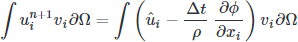
Next, we adjust how the “tentative velocity” is updated during each simulation step. This field represents the approximated velocity at the next time step, ignoring pressure (as it’s still unknown at this point). Here’s where we replace the Chorin split method with the Kim and Moin fractional step method. In other words, we modify the expression for the field F1:

Replace:

 1
 2
 3
 4
 5
 6
 7
 8
 9
10
11

# Tentative velocity field (a first prediction of what the next velocity field is)
# for the Chorin style split
# F1 = change in the velocity field +
#      convective term +
#      diffusive term -
#      body force term

F1 = (1/k)*inner(u - u0, v)*dx + \
     inner(grad(u0)*u0, v)*dx + \
     nu*inner(grad(u), grad(v))*dx - \
     inner(f, v)*dx

With:

 1
 2
 3
 4
 5
 6
 7
 8
 9
10
11

# Tentative velocity field (a first prediction of what the next velocity field is)
# for the Kim and Moin style split
# F1 = change in the velocity field +
#      convective term +
#      diffusive term -
#      body force term

F1 = (1/k)*inner(u - u0, v)*dx + \ 
     (3.0/2.0) * inner(grad(u0)*u0, v)*dx - (1.0/2.0) * inner(grad(un1)*un1, v)*dx + \ 
     (nu/2.0)*inner(grad(u+u0), grad(v))*dx - \ 
     inner(f, v)*dx 

Now, the demo employs our updated method to solve for the intermediate velocity field using F1.

Lastly, we ensure that the previous velocity field, un1, is updated at the end of each iteration step:

1
2
3
4
5

...
# Move to next time step
un1.assign(u0)		# copy the current velocity field into the previous velocity field
u0.assign(u1)		# copy the next velocity field into the current velocity field
...

Below is the complete code for our FEniCS CFD demo, including our changes:

  1
  2
  3
  4
  5
  6
  7
  8
  9
 10
 11
 12
 13
 14
 15
 16
 17
 18
 19
 20
 21
 22
 23
 24
 25
 26
 27
 28
 29
 30
 31
 32
 33
 34
 35
 36
 37
 38
 39
 40
 41
 42
 43
 44
 45
 46
 47
 48
 49
 50
 51
 52
 53
 54
 55
 56
 57
 58
 59
 60
 61
 62
 63
 64
 65
 66
 67
 68
 69
 70
 71
 72
 73
 74
 75
 76
 77
 78
 79
 80
 81
 82
 83
 84
 85
 86
 87
 88
 89
 90
 91
 92
 93
 94
 95
 96
 97
 98
 99
100
101
102
103
104
105
106
107
108
109
110
111
112
113
114
115
116
117
118
119
120
121
122
123
124
125
126
127
128
129

"""This demo program solves the incompressible Navier-Stokes equations
on an L-shaped domain using Kim and Moin's fractional step method."""

# Begin demo

from dolfin import *

# Print log messages only from the root process in parallel
parameters["std_out_all_processes"] = False;

# Load mesh from file
mesh = Mesh("lshape.xml.gz")

# Define function spaces (P2-P1)
V = VectorFunctionSpace(mesh, "Lagrange", 2)
Q = FunctionSpace(mesh, "Lagrange", 1)

# Define trial and test functions
u = TrialFunction(V)
p = TrialFunction(Q)
v = TestFunction(V)
q = TestFunction(Q)

# Set parameter values
dt = 0.01
T = 3
nu = 0.01

# Define time-dependent pressure boundary condition
p_in = Expression("sin(3.0*t)", t=0.0)

# Define boundary conditions
noslip  = DirichletBC(V, (0, 0),
                      "on_boundary && \
                       (x[0] < DOLFIN_EPS | x[1] < DOLFIN_EPS | \
                       (x[0] > 0.5 - DOLFIN_EPS && x[1] > 0.5 - DOLFIN_EPS))")
inflow  = DirichletBC(Q, p_in, "x[1] > 1.0 - DOLFIN_EPS")
outflow = DirichletBC(Q, 0, "x[0] > 1.0 - DOLFIN_EPS")
bcu = [noslip]
bcp = [inflow, outflow]

# Create functions
un1 = Function(V)
u0 = Function(V)
u1 = Function(V)
p1 = Function(Q)

# Define coefficients
k = Constant(dt)
f = Constant((0, 0))

# Tentative velocity field (a first prediction of what the next velocity field is)
# for the Kim and Moin style split
# F1 = change in the velocity field +
#     convective term +
#     diffusive term -
#     body force term

F1 = (1/k)*inner(u - u0, v)*dx + \
     (3.0/2.0) * inner(grad(u0)*u0, v)*dx - (1.0/2.0) * inner(grad(un1)*un1, v)*dx + \
     (nu/2.0)*inner(grad(u+u0), grad(v))*dx - \
     inner(f, v)*dx 
a1 = lhs(F1)
L1 = rhs(F1)

# Pressure update
a2 = inner(grad(p), grad(q))*dx
L2 = -(1/k)*div(u1)*q*dx

# Velocity update
a3 = inner(u, v)*dx
L3 = inner(u1, v)*dx - k*inner(grad(p1), v)*dx

# Assemble matrices
A1 = assemble(a1)
A2 = assemble(a2)
A3 = assemble(a3)

# Use amg preconditioner if available
prec = "amg" if has_krylov_solver_preconditioner("amg") else "default"

# Create files for storing solution
ufile = File("results/velocity.pvd")
pfile = File("results/pressure.pvd")

# Time-stepping
t = dt
while t < T + DOLFIN_EPS:

    # Update pressure boundary condition
    p_in.t = t

    # Compute tentative velocity step
    begin("Computing tentative velocity")
    b1 = assemble(L1)
    [bc.apply(A1, b1) for bc in bcu]
    solve(A1, u1.vector(), b1, "gmres", "default")
    end()

    # Pressure correction
    begin("Computing pressure correction")
    b2 = assemble(L2)
    [bc.apply(A2, b2) for bc in bcp]
    solve(A2, p1.vector(), b2, "cg", prec)
    end()

    # Velocity correction
    begin("Computing velocity correction")
    b3 = assemble(L3)
    [bc.apply(A3, b3) for bc in bcu]
    solve(A3, u1.vector(), b3, "gmres", "default")
    end()

    # Plot solution
    plot(p1, title="Pressure", rescale=True)
    plot(u1, title="Velocity", rescale=True)

    # Save to file
    ufile << u1
    pfile << p1

    # Move to next time step
    un1.assign(u0)
    u0.assign(u1)
    t += dt
    print "t =", t

# Hold plot
interactive()

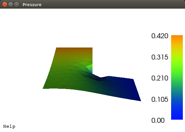
Running the program reveals the flow around the elbow. I encourage you to run the scientific computing code yourself to see the animation! Screenshots of the final frame are shown below.

Relative pressures in the bend at the end of the simulation, scaled and colored by magnitude (non-dimensional values):

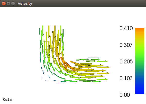
Relative velocities in the bend at the end of the simulation as vector glyphs scaled and colored by magnitude (non-dimensional values).

In essence, we took an existing demo with a scheme similar to ours and modified it to utilize better approximations by incorporating information from the previous time step.

You might be thinking that was a simple edit. It was, and that’s precisely the point. This open-source scientific computing project enabled us to swiftly implement a modified numerical model by changing just four lines of code. Similar changes in extensive research codes could take months.

The project provides many other demos that can serve as starting points. There are even several open source applications built upon the project, implementing various models.

Conclusion

While scientific computing and its applications are undeniably complex, the ever-expanding landscape of open-source tools and projects can significantly streamline what would otherwise be daunting programming tasks. Perhaps the day is approaching when scientific computing becomes accessible enough for widespread adoption beyond the research community.

APPENDIX: Scientific and Mathematical Underpinnings

This appendix delves into the technical details behind the Computational Fluid Dynamics guide above. It serves as a concise summary of topics typically covered in numerous graduate-level courses and can be particularly insightful for graduate students and those interested in the mathematical intricacies of the subject.

Fluid Mechanics

“Modeling” generally refers to the process of approximating real-world systems. Models often involve continuous equations that are challenging to implement computationally and thus require further approximation using numerical methods.

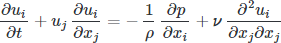
For fluid mechanics, we begin with the foundational equations, the Navier-Stokes equations, as a starting point for developing a CFD scheme.

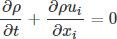
The Navier-Stokes equations are a set of partial differential equations (PDEs) that effectively describe fluid flows. These equations arise from applying conservation laws of mass, momentum, and energy, combined with a Reynolds Transport Theorem, Gauss’s theorem, and Stoke’s Hypothesis. They rely on a continuum assumption, which presumes enough fluid particles to define statistical properties like temperature, density, and velocity. Furthermore, assumptions of a linear relationship between stress and strain rate tensors, symmetry in the stress tensor, and an isotropic fluid are also required. Understanding these assumptions is crucial for evaluating the resulting code’s applicability. Without further ado, here are the Navier-Stokes equations in Einstein notation:

Conservation of mass:

Conservation of momentum:

Conservation of energy:

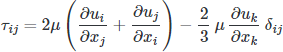
where the deviatoric stress is given by:

While these equations are very general and govern most real-world fluid flows, they are not directly practical. Few exact solutions to these equations are known, and a $1,000,000 Millennium Prize awaits anyone who can solve the existence and smoothness problem. Nevertheless, they provide a starting point for model development by introducing simplifying assumptions to reduce complexity (they are among the most challenging equations in classical physics).

To simplify, we leverage domain-specific knowledge to make an incompressible assumption for the fluid and assume constant temperatures. Consequently, we can disregard the conservation of energy equation (which becomes the heat equation) as it becomes decoupled. This leaves us with two equations, still PDEs, but significantly simpler while remaining relevant to a wide range of fluid problems.

Continuity equation:

Momentum equations:

Now, we have a suitable mathematical model for incompressible fluid flows (e.g., low-speed gases and liquids like water). Although not straightforward, these equations allow for obtaining “exact” solutions for simple problems. Addressing more complex scenarios, like airflow over a wing or water flow through a system, necessitates numerical solutions.

Building a Numerical Scheme

To tackle intricate problems computationally, we need a method to numerically solve our incompressible flow equations. This task is not trivial, and our equations present a particular challenge: solving the momentum equations while ensuring a divergence-free solution, as mandated by the continuity equation. Simple time integration methods, such as Runge-Kutta method, become tricky due to the absence of a time derivative in the continuity equation.

No single “correct” or “best” method exists for solving these equations, but numerous viable options are available. Over time, various approaches have emerged to address this challenge, including reformulating the equations in terms of vorticity and stream-function, introducing artificial compressibility, and employing operator splitting techniques. Chorin (1969), followed by Kim and Moin (1984, 1990), developed a highly successful and popular fractional step method. This method enables integrating the equations while directly solving for the pressure field instead of resorting to implicit solutions. The fractional step method, a general approach for approximating equations by splitting their operators (in this case, splitting along pressure), offers relative simplicity and robustness, motivating its use here.

First, we need to discretize the equations in time numerically, allowing us to advance from one time point to the next. Following Kim and Moin (1984), we’ll use the second-order-explicit Adams-Bashforth method for convective terms, the second-order-implicit Crank-Nicholson method for viscous terms, a simple finite difference for the time derivative, and neglect the pressure gradient. These choices are not unique; their selection is part of the art of constructing a numerically well-behaved scheme.

While this allows for integrating the intermediate velocity, it disregards the pressure contribution and results in a non-divergence-free solution (incompressibility requires it to be divergence-free). The remaining part of the operator is needed to reach the next time step.

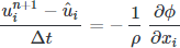
where

is a scalar value that needs to be determined to ensure a divergence-free velocity. We can find

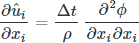
by taking the divergence of the correction step.

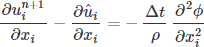
The first term becomes zero as per the continuity equation, yielding a Poisson equation for a scalar field that will provide a solenoidal (divergence-free) velocity at the next time step.

As demonstrated by Kim and Moin (1984),

is not precisely the pressure due to the operator splitting. However, it can be obtained using

.

At this stage, we have successfully discretized the governing equations in time, enabling their integration. Next, we need to discretize the operators spatially. Several methods can achieve this, including the Finite Element Method, the Finite Volume Method, and the Finite Difference Method. In their original work, Kim and Moin (1984) employed the Finite Difference Method. While advantageous for its relative simplicity and computational efficiency, it struggles with complex geometries, requiring a structured mesh.

We opt for the Finite Element Method (FEM) due to its generality and the availability of excellent open-source projects that facilitate its use. FEM effectively handles real geometries in one, two, and three dimensions, scales well to large problems on computer clusters, and is relatively straightforward to use with high-order elements. Although typically slower than the other methods mentioned, its versatility across problems makes it a suitable choice for this guide.

Even within the FEM framework, numerous choices exist. Here, we will utilize the Galerkin FEM, which involves casting the equations in weighted residual form by multiplying each by a test function -

for vectors and

for the scalar field - and integrating over the domain

. We then perform partial integration on higher-order derivatives using Stoke’s theorem or the Divergence theorem. Finally, we pose the variational problem, leading to our desired CFD scheme.

Now, we have a well-defined mathematical scheme in a form suitable for implementation, with some understanding of the steps involved (a considerable amount of mathematics and methods borrowed from brilliant researchers).