This piece explores how to use Python to build a system capable of making real-time predictions using machine learning or artificial intelligence (AI). We’ll be employing a Flask REST API to achieve this. This architecture can be seen as a stepping stone for taking machine learning applications from the proof of concept (PoC) stage to a minimal viable product (MVP).

When aiming for real-time solutions, Python might not be the first tool that comes to mind. However, the extensive use of Python libraries like Tensorflow and Scikit-Learn in the field of machine learning makes it a convenient choice for numerous Jupyter Notebook PoCs.

The feasibility of this solution hinges on the fact that training a model demands significantly more time than generating a prediction. Think of it like watching a movie: comprehending the content (training) is time-consuming, but answering questions about it afterward (predicting) is relatively quick. There’s no need to rewatch the entire film for each question.

Training essentially creates a condensed representation of the “movie,” and predicting involves retrieving information from this compressed form. This retrieval process should be rapid, regardless of the movie’s length or complexity.

Let’s illustrate this with a straightforward Python example using the Flask framework.

A Typical Machine Learning Architecture

To begin, let’s outline the general flow of a training and prediction architecture:

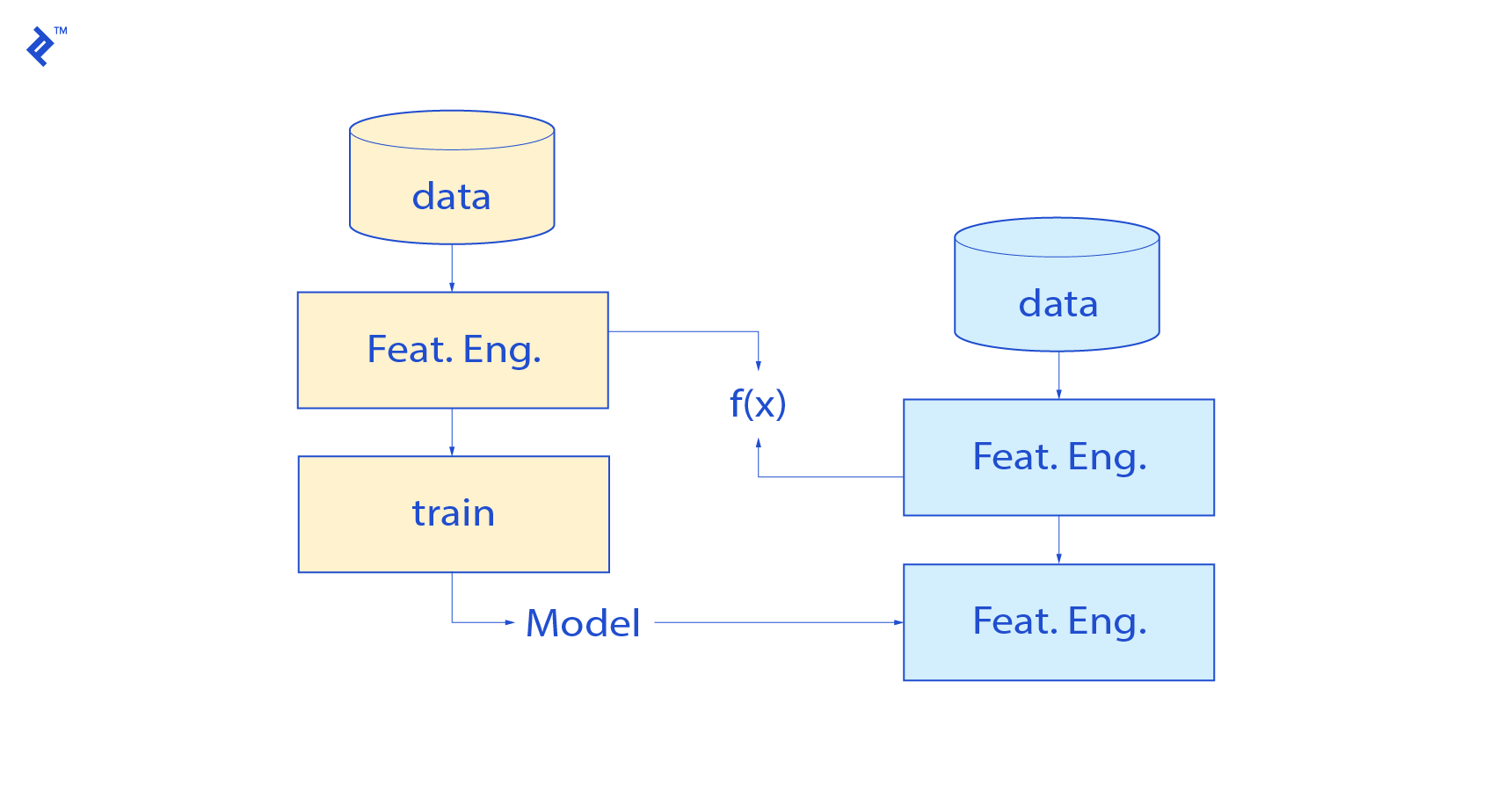
Initially, a training pipeline is established. Its purpose is to analyze historical data and extract patterns in line with a defined objective function.

This pipeline yields two crucial components:

1. Feature engineering functions: These are the transformations applied to the data during training. It’s essential to reapply these same transformations when making predictions.
2. Model parameters: This encompasses the chosen algorithm, its settings (hyperparameters), and any learned weights. These parameters need to be stored for consistent prediction.

It’s critical to meticulously store the feature engineering steps performed during training to ensure they are correctly applied during prediction. One common challenge is feature scaling, which is essential for the proper functioning of many algorithms.

For instance, if feature X1 initially ranges from 1 to 1000 and is then scaled to a range of [0,1] using the function f(x) = x/max(X1), what happens when a new data point to be predicted has a value of 2000 for X1?

Carefully designed adjustments are needed in the mapping function to handle such scenarios, ensuring that outputs remain consistent and are correctly calculated during prediction.

Machine Learning: Training vs. Predicting

A fundamental question arises: Why separate training and prediction in the first place?

In the controlled environments of machine learning tutorials and examples, where the entire dataset (including the data to be predicted) is known beforehand, the simplest approach is to combine training and prediction data into a single dataset (often with a designated “test set”).

The model is trained on the “training set” and evaluated on the “test set” to assess its performance. Feature engineering is applied to both sets within the same pipeline.

However, real-world systems don’t usually provide all the data upfront. Training data is readily available, but the data requiring predictions arrives continuously, similar to watching a movie once and then being asked questions about it later. The answers need to be generated efficiently and rapidly.

Furthermore, retraining the entire model every time new data arrives is often impractical. Training can be time-intensive (potentially taking weeks for large image datasets) and the model should ideally remain stable over time.

This is why separating training and prediction is often beneficial, and in many systems, even essential. This approach aligns more closely with how intelligent systems (whether artificial or biological) acquire and apply knowledge.

The Link to Overfitting

Decoupling training and prediction also helps address the issue of overfitting.

In statistical modeling, overfitting occurs when an analysis fits the training data too closely. This often results in poor generalization to new, unseen data, making the model less reliable for making predictions on data it hasn’t encountered before.

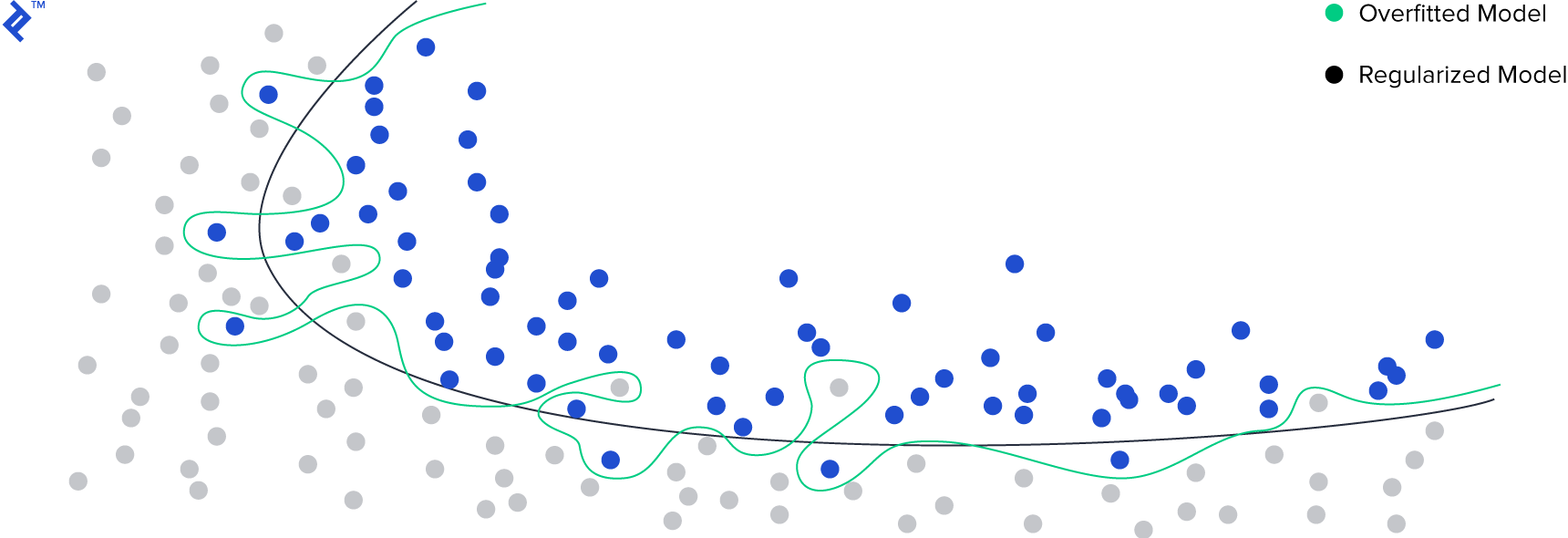
Overfitting is especially common in datasets with numerous features or limited training examples. In these scenarios, the model might identify spurious patterns in the training data that don’t reflect true underlying relationships. It’s akin to mistaking noise for a meaningful signal.

A key method for mitigating overfitting is to divide the data into separate sets for training and evaluation. This allows us to assess how well the model generalizes to unseen data. The error observed on the evaluation set (which the model has not been trained on) provides a more realistic estimate of how the model is likely to perform on new data in a real-world setting.

By carefully designing our training and prediction pipeline and implementing a suitable data splitting strategy, we not only address overfitting but also establish a robust architecture for making predictions on new, unseen data.

A final, crucial step is to continuously monitor the model’s performance on new data to ensure that the error remains within acceptable bounds. While some degree of performance difference between the evaluation set and real-world data is expected, this difference should be manageable. Monitoring and managing this performance gap is an ongoing process, but delving into its specifics is beyond the scope of this article.

Predicting with a REST API

This is where the clear separation between training and prediction becomes particularly advantageous. Having saved our feature engineering methods and model parameters, we can construct a straightforward REST API that leverages these components.

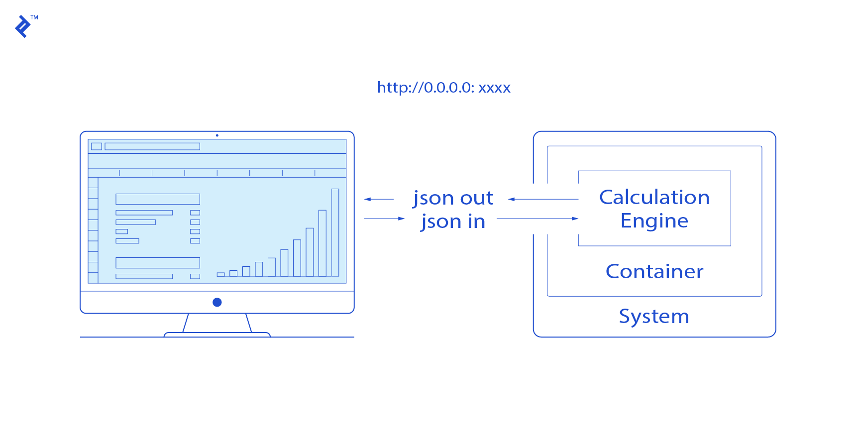
The crucial aspect is to load the trained model and its parameters when the API is initialized. Once loaded and residing in memory, each API call triggers two actions:

1. The feature engineering calculations are applied to the incoming data.
2. The ‘predict’ function of our trained machine learning algorithm is executed on the transformed data.

Both of these operations are usually swift enough to guarantee a real-time response.

The API can be designed to accept either single or multiple data points for prediction (batch predictions).

Below is a minimal Python/Flask code snippet illustrating this principle. It outlines a basic API that accepts a JSON input (representing a question or request) and returns a JSON output (the model’s answer or prediction):

 1
 2
 3
 4
 5
 6
 7
 8
 9
10
11
12
13
14
15
16
17
18
19
20
21
22
23
24
25
26
27
28
29
30
31
32
33
34
35
36
37
38
39
40
41
42

app = Flask(__name__)

@app.route('/api/makecalc/', methods=['POST'])

def makecalc():

	"""

	Function run at each API call

        No need to re-load the model 

    

	"""

        # reads the received json 

	jsonfile = request.get_json()

	res = dict()

	for key in jsonfile.keys():

            # calculates and predicts 

    	    res[key] = model.predict(doTheCalculation(key))

   	

	# returns a json file 

	return jsonify(res)

if __name__ == '__main__':

        # Model is loaded when the API is launched

	model = pickle.load(open('modelfile', 'rb'))

	app.run(debug=True)

While this API is well-suited for generating predictions from new data, I advise against using it directly for training the model. While technically feasible, it introduces complexities into the training code and could lead to increased memory demands, especially when dealing with large datasets or computationally intensive models.

A Practical Example: Bike Sharing

Let’s consider a real-world scenario using the “Bike Sharing” dataset from Kaggle. Imagine we operate a bike-sharing company aiming to predict the daily demand for bike rentals to optimize bike maintenance, logistics, and other business operations.

Bike rentals are heavily influenced by weather conditions. By integrating weather forecasts into our model, we can anticipate periods of peak demand and proactively schedule maintenance during less busy times, minimizing disruptions to service and maximizing bike availability.

Firstly, we train a machine learning model and save it as a pickle file. You can find the code for this in the Jupyter notebook.

For this illustration, we won’t delve into the specifics of model training and evaluation, as our focus is on understanding the entire workflow.

Next, we define the data transformation logic to be applied each time the API is called:

 1
 2
 3
 4
 5
 6
 7
 8
 9
10
11
12
13
14
15
16
17
18
19
20

import numpy as np

import pandas as pd

from datetime import date

def doTheCalculation(data):

	data['dayofyear']=(data['dteday']-

    	data['dteday'].apply(lambda x: date(x.year,1,1))

    	.astype('datetime64[ns]')).apply(lambda x: x.days)

	X = np.array(data[['instant','season','yr','holiday','weekday','workingday',

                  	'weathersit','temp','atemp','hum','windspeed','dayofyear']])

	return X

In this simplified example, we engineer a new feature (“day of year”) by combining the month and day information. We also select and order the relevant columns to be fed into our model.

With the data transformation defined, we proceed to create the REST API using Flask:

 1
 2
 3
 4
 5
 6
 7
 8
 9
10
11
12
13
14
15
16
17
18
19
20
21
22
23
24
25
26
27
28
29
30
31
32
33
34
35
36
37
38
39
40
41
42
43
44
45
46
47
48
49
50

from flask import Flask, request, redirect, url_for, flash, jsonify

from features_calculation import doTheCalculation

import json, pickle

import pandas as pd

import numpy as np

app = Flask(__name__)

@app.route('/api/makecalc/', methods=['POST'])

def makecalc():

	"""

	Function run at each API call

	"""

	jsonfile = request.get_json()

	data = pd.read_json(json.dumps(jsonfile),orient='index',convert_dates=['dteday'])

	print(data)

	res = dict()

	ypred = model.predict(doTheCalculation(data))

	for i in range(len(ypred)):

    	    res[i] = ypred[i]

    

	return jsonify(res) 

if __name__ == '__main__':

	modelfile = 'modelfile.pickle'    

	model = pickle.load(open(modelfile, 'rb'))

	print("loaded OK")

	app.run(debug=True)

Executing this code will start a local server, making our API accessible at the default port 5000.

We can test the API locally using Python:

 1
 2
 3
 4
 5
 6
 7
 8
 9
10

import requests, json

url = '[http://127.0.0.1:5000/api/makecalc/](http://127.0.0.1:5000/api/makecalc/)'

text = json.dumps({"0":{"instant":1,"dteday":"2011-01-01T00:00:00.000Z","season":1,"yr":0,"mnth":1,"holiday":0,"weekday":6,"workingday":0,"weathersit":2,"temp":0.344167,"atemp":0.363625,"hum":0.805833,"windspeed":0.160446},

               	"1":{"instant":2,"dteday":"2011-01-02T00:00:00.000Z","season":1,"yr":0,"mnth":1,"holiday":0,"weekday":3,"workingday":0,"weathersit":2,"temp":0.363478,"atemp":0.353739,"hum":0.696087,"windspeed":0.248539},

               	"2":{"instant":3,"dteday":"2011-01-03T00:00:00.000Z","season":1,"yr":0,"mnth":1,"holiday":0,"weekday":1,"workingday":1,"weathersit":1,"temp":0.196364,"atemp":0.189405,"hum":0.437273,"windspeed":0.248309}})

The request payload contains all the necessary information our model expects to generate predictions. Our model will process this information and respond with a forecast of bike rentals for the specified dates (in this case, three different dates).

 1
 2
 3
 4
 5
 6
 7
 8
 9
10

headers = {'content-type': 'application/json', 'Accept-Charset': 'UTF-8'}
r = requests.post(url, data=text, headers=headers)
print(r,r.text)

<Response [200]> {
  "0": 1063, 
  "1": 1028, 
  "2": 1399
}

And that’s it! This simple yet powerful service can be easily integrated into various applications within the company. It can inform maintenance schedules, provide insights to users about anticipated bike traffic and demand, and enhance the overall efficiency of bike rental operations.

Bringing it All Together

A common pitfall in many machine learning systems, particularly during the PoC phase, is the entanglement of training and prediction.

By consciously separating these two phases, we can construct systems capable of delivering real-time predictions with relative ease. This approach, utilizing Python and Flask alongside popular machine learning libraries like Scikit-learn or TensorFlow, offers a cost-effective and efficient pathway for developing MVPs, especially when starting from existing PoC implementations.

While this architecture is broadly applicable, it’s worth noting that certain applications might present challenges. For instance, scenarios involving complex or resource-intensive feature engineering or those requiring the very latest data for each prediction (e.g., finding the closest match in a constantly updating database) might necessitate alternative approaches.

In essence, just as you wouldn’t rewatch an entire movie to answer a simple question, the same principle applies to machine learning. Efficiency lies in separating the learning phase from the application of that learned knowledge.