In the current data-driven world, researchers are heavily focused on data to answer interesting questions. The sheer volume of data presents a significant obstacle to processing and analysis, especially for statisticians and data analysts who lack the time to master business intelligence platforms or technologies within the Hadoop ecosystem, Spark, or NoSQL databases, despite their ability to facilitate rapid analysis of terabytes of data.

Currently, it’s common for researchers and statisticians to develop models using data subsets within analytics tools such as R, MATLAB, or Octave. Subsequently, they provide the formulas and data processing instructions to IT teams, who then construct production analytics solutions.

A drawback of this method is the need to repeat the entire process if the researcher uncovers new insights after running the model on the complete production dataset.

Consider a scenario where a researcher could collaborate with a MongoDB developer to perform analysis directly on the entire production dataset, treating it as an exploratory dataset, all without requiring knowledge of new technologies, complex programming languages, or even SQL.

By effectively utilizing MongoDB’s Aggregation Pipeline and MEAN, we can accomplish this within a reasonable timeframe. This article, along with the accompanying code here in this GitHub repository, aims to demonstrate the ease with which this can be achieved.

While many available Business Intelligence tools allow researchers to import datasets from NoSQL and other Big Data technologies for in-tool transformation and analysis, our approach in this tutorial leverages the capabilities of the MongoDB Aggregation Pipeline. This eliminates the need to extract data from MongoDB, empowering researchers to perform diverse transformations on a production big data system through a user-friendly interface.

MongoDB Aggregation Pipeline for Business Intelligence

In simple terms, the MongoDB aggregation pipeline is a framework for executing a sequence of data transformations on a dataset. The initial stage operates on the entire collection of documents, while each subsequent stage takes the output of the preceding transformation as input, producing a transformed output.

Ten types of transformations can be employed within an aggregation pipeline:

• $geoNear: Orders documents based on their proximity to a specified point, from nearest to farthest.

• $match: Filters the input record set using specified expressions.

• $project: Generates a result set containing a subset of input fields or computed fields.

• $redact: Restricts document content based on information within the document.

• $unwind: Expands an array field with n elements from a document into n documents, each containing one element from the array as a field, replacing the original array.

• $group: Groups documents based on one or more columns and performs aggregations on other columns.

• $limit: Selects the first n documents from the input set (useful for percentile calculations, etc.).

• $skip: Disregards the first n documents from the input set.

• $sort: Sorts all input documents according to the provided object.

• $out: Writes all documents from the previous stage to a collection.

Apart from the first and last transformations listed, there are no restrictions on the order in which these transformations can be applied. The $out stage should be used only once and at the end of the pipeline if the goal is to store the result in a new or existing collection. The $geoNear stage can only be used as the initial stage of a pipeline.

To illustrate these concepts, let’s examine two datasets and address two questions related to them.

Salary Discrepancies by Designation

To showcase the capabilities of the MongoDB aggregation pipeline, we’ll utilize a dataset containing salary information for university instructional staff across the United States, available at nces.ed.gov. The dataset encompasses data from 7,598 institutions and includes the following fields:

 1
 2
 3
 4
 5
 6
 7
 8
 9
10
11
12
13
14
15

var FacultySchema = mongoose.Schema({
	InstitutionName : String,
	AvgSalaryAll : Number,
	AVGSalaryProfessors : Number,
	AVGSalaryAssociateProfessors : Number,
	AVGSalaryAssistantProfessors : Number,
	AVGSalaryLecturers : Number,
	AVGSalaryInstructors : Number,
	StreetAddress : String,
	City : String,
	State : String,
	ZIPCode : String,
	MenStaffCount : Number,
	WomenStaffCount : Number
}

Our objective is to determine the average salary difference between associate professors and professors by state, allowing an associate professor to assess their relative salary standing compared to professors in different states.

Initially, we need to cleanse the dataset by removing invalid entries where the average salary is either null or an empty string. This is accomplished using the following stage:

1

{$match: {AVGSalaryProfessors: {$not: {$type: 2}}, AVGSalaryAssociateProfessors:  {$not: {$type: 2}}}}

This stage filters out any records containing string values in the specified fields. In MongoDB, each type is represented by a represented with a unique number - for strings, the type number is 2.

This dataset exemplifies real-world data analytics challenges, where data cleansing is often a necessary step.

With a clean dataset, we can proceed to calculate the average salaries by state:

1

{$group: {_id: "$State", StateAVGSalaryProfessors: {$avg: "$AVGSalaryProfessors"}, StateAVGSalaryAssociateProfessors: {$avg: "$AVGSalaryAssociateProfessors"}}}

Next, we project the results to obtain the difference in average salaries between states:

1

{$project: {_ID: 1, SalaryDifference: {$subtract: ["$StateAVGSalaryProfessors", "$StateAVGSalaryAssociateProfessors"]}}}

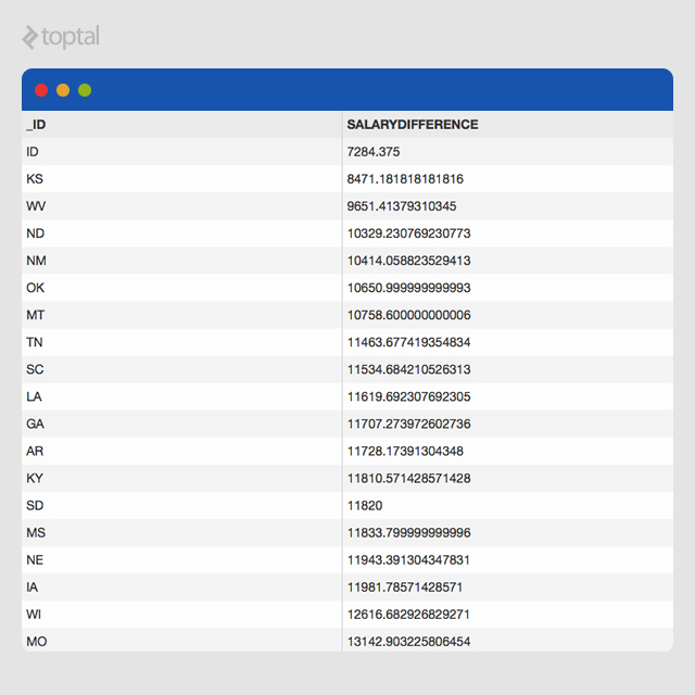
This provides the average salary difference between professors and associate professors at the state level, based on data from 7,519 educational institutions across the US. To enhance interpretability, we can sort the results to identify states with the smallest differences:

1

{$sort: { SalaryDifference: 1}}

Based on this dataset, Idaho, Kansas, and West Virginia exhibit the smallest salary discrepancies between associate professors and professors compared to other states.

The complete aggregation pipeline for this analysis is presented below:

1
2
3
4
5
6

[
{$match: {AVGSalaryProfessors: {$not: {$type: 2}}, AVGSalaryAssociateProfessors:  {$not: {$type: 2}}}},
{$group: {_id: "$State", StateAVGSalaryProfessors: {$avg: "$AVGSalaryProfessors"}, StateAVGSalaryAssociateProfessors: {$avg: "$AVGSalaryAssociateProfessors"}}},
{$project: {_ID: 1, SalaryDifference: {$subtract: ["$StateAVGSalaryProfessors", "$StateAVGSalaryAssociateProfessors"]}}},
{$sort: { SalaryDifference: 1}}
]

The resulting dataset is displayed below. Researchers can export these results to a CSV file for further analysis and visualization using tools like Tableau or Microsoft Excel.

Average Pay by Employment Type

Let’s explore another example using a dataset from www.data.gov containing payroll information for state and local government employees in the US. Our goal is to determine the average pay for full-time and part-time “Financial Administration” employees in each state.

After importing the dataset, we have 1,975 documents, each adhering to the following schema:

 1
 2
 3
 4
 5
 6
 7
 8
 9
10
11
12
13

mongoose.Schema({
	State : String,
	GovernmentFunction : String,
	FullTimeEmployees : Number,
	VariationPCT : Number,
	FullTimePay : Number,
	PartTimeEmployees : Number,
	PartTimePay : Number,
	PartTimeHours : Number,
	FullTimeEquivalentEmployment : Number,
	TotalEmployees : Number,
	TotalMarchPay : Number
	}, {collection: 'payroll'});

The answer to this question could assist “Financial Administration” employees in identifying the most lucrative states. Our MongoDB aggregation pipeline tool facilitates this analysis:

First, we filter the dataset based on the “GovernmentFunction” column to exclude non-“Financial Administration” entries:

1

{$match:{GovernmentFunction:'Financial Administration'}}

Next, we group the entities by state and compute the average full-time and part-time salaries for each state:

1

{$group: {_id: '$State', FTP_AVG: {$avg: '$FullTimePay'}, PTM_AVG: {$avg: '$PartTimePay'}}}

Finally, we sort the results in descending order of average pay:

1

{$sort: {FTP_AVG: -1, PTM_AVG: -1}}

This generates the following aggregation pipeline:

1
2
3
4
5

[
    {$match:{GovernmentFunction:'Financial Administration'}},
    {$group: {_id: '$State', FTP_AVG: {$avg: '$FullTimePay'}, PTM_AVG: {$avg: '$PartTimePay'}}},
    {$sort: {FTP_AVG: -1, PTM_AVG: -1}}
]

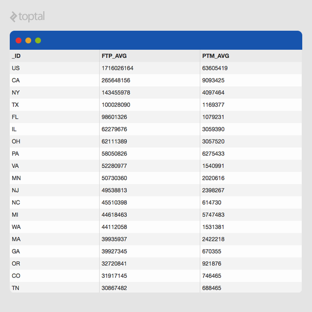
Executing the aggregation pipeline produces the following results:

Building Blocks

This business intelligence application leverages MEAN, a combination of MongoDB, ExpressJS, AngularJS, and NodeJS.

MongoDB, as you may know, is a schemaless document database. Despite the 16MB size limit per document, its flexibility, performance, and the powerful aggregation pipeline framework make it an ideal choice for this tool. Getting started with MongoDB is straightforward thanks to its comprehensive documentation.

Node.js, another crucial component of the MEAN stack, provides an event-driven, server-side JavaScript environment powered by Google Chrome’s V8 engine. The scalability potential of Node.js is attracting significant interest from many organizations.

Express.js, the most popular web application framework for Node.js, simplifies the creation of APIs and other server-side business logic for web applications. Its minimalist design ensures speed and flexibility.

AngularJS, developed and maintained by Google engineers, is rapidly gaining popularity as a front-end JavaScript framework.

The MEAN stack’s popularity, and our preference for application development at techXplorers, stems from two key factors:

• Simplified Skillset: Proficiency in JavaScript is sufficient for all layers of the application.

• JSON-Based Communication: Communication between the front-end, business logic, and database layers occurs through JSON objects, streamlining design and development across layers.

Conclusion

This MongoDB aggregation pipeline tutorial has demonstrated a cost-effective approach to empowering researchers with a tool that utilizes production data as an exploratory dataset. This enables researchers to perform various transformations, conduct analysis, and build models.

Our team of four experienced engineers (two in the US and two in India), along with a designer and freelance UX expert, developed and deployed this application in just three days. In a future article, I’ll elaborate on how this level of collaboration enables the creation of exceptional products within incredibly short timeframes.

We encourage you to explore the capabilities of the MongoDB Aggregation Pipeline and empower your researchers to unlock valuable insights from your data.

You can experiment with this live application at here.