In a recent article on Toptal’s blog, data science expert Charles Cook provided insights into scientific computing using open-source tools. His guide highlights the significance of these tools in simplifying data processing and result acquisition.

However, once we’ve tackled those intricate differential equations, a new challenge emerges: comprehending and interpreting the massive datasets generated by these simulations. How can we visualize potentially gigabytes of data, such as those containing millions of grid points from a large simulation?

While working on similar issues for my Master’s Thesis, I discovered the Visualization Toolkit (VTK), a powerful graphics library specifically designed for data visualization.

This tutorial offers a concise introduction to VTK and its pipeline architecture, followed by a practical 3D visualization example using data from a simulated fluid in an impeller pump. Lastly, I’ll highlight the library’s strengths and the limitations I’ve come across.

Data Visualization and The VTK Pipeline

The open-source library VTK features a robust processing and rendering pipeline equipped with numerous advanced visualization algorithms. Its capabilities extend beyond visualization, encompassing image and mesh processing algorithms added over time. In my current endeavor with a dental research firm, I’m employing VTK for mesh-based processing within a Qt-based, CAD-like software. The VTK case studies demonstrate the wide spectrum of suitable applications.

VTK’s architecture revolves around a powerful pipeline concept, illustrated below:

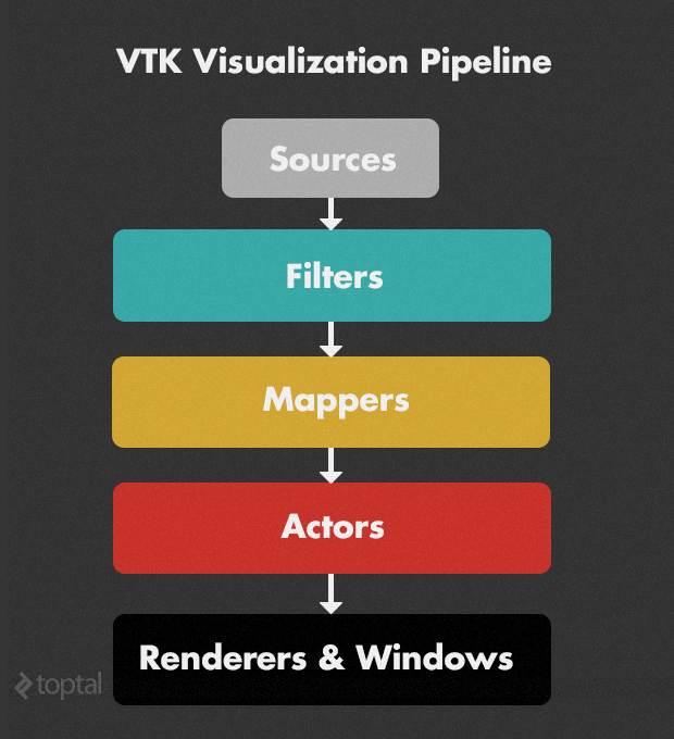
• Sources initiate the pipeline by creating data from scratch. For instance, vtkConeSource generates a 3D cone, while vtkSTLReader imports *.stl 3D geometry files.
• Filters transform the output of sources or other filters, creating modified data. An example is vtkCutter, which slices the preceding object using an implicit function, like a plane. VTK’s processing algorithms are implemented as filters that can be seamlessly chained together.
• Mappers convert data into graphical elements, such as specifying a color lookup table for scientific data, providing an abstract way to define visual representations.
• Actors represent objects (geometry and display attributes) within the scene, defining properties like color, opacity, shading, and orientation.
• Renderers & Windows handle the platform-independent rendering onto the screen.

A typical VTK rendering pipeline begins with one or more sources, applies various filters to process them into multiple outputs, which are then rendered individually using mappers and actors. This concept’s strength lies in its update mechanism. Modifying filter or source settings automatically updates all dependent filters, mappers, actors, and render windows. Conversely, objects further down the pipeline can easily retrieve necessary information.

Furthermore, direct interaction with rendering systems like OpenGL is unnecessary. VTK abstracts low-level tasks in a platform- and (partially) rendering system-independent manner, enabling developers to work at a higher level.

Code Example with a Rotor Pump Dataset

Let’s delve into a data visualization example using a dataset from the IEEE Visualization Contest 2011, showcasing fluid flow in a rotating impeller pump. This data originates from a computational fluid dynamics simulation, similar to the one detailed in Charles Cook’s article.

The zipped simulation data for the featured pump exceeds 30 GB, comprising multiple parts and time steps, contributing to its size. This guide focuses on the rotor part from a single time step, with a compressed size of approximately 150 MB.

I prefer using C++ with VTK, although mappings for languages like Tcl/Tk, Java, and Python exist. If the goal is solely to visualize a single dataset, coding is optional, thanks to Paraview, a graphical interface for most VTK functions.

The Dataset and Why 64-bit is Necessary

I extracted the rotor dataset from the 30 GB dataset by opening a time step in Paraview and saving the rotor part separately. The result is an unstructured grid file, representing a 3D volume composed of points and 3D cells like hexahedra and tetrahedra. Each 3D point has associated values, while cells may or may not have them (not in this case). This tutorial focuses on visualizing pressure and velocity at the points within their 3D context.

The compressed file size is around 150 MB, expanding to 280 MB in memory when loaded with VTK. However, VTK’s processing leads to multiple dataset caching within the pipeline, quickly reaching the 2 GB memory limit for 32-bit programs. While memory-saving techniques exist in VTK, this example will be compiled and run in 64-bit for simplicity.

Acknowledgements: The dataset is courtesy of the Institute of Applied Mechanics, Clausthal University, Germany (Dipl. Wirtsch.-Ing. Andreas Lucius).

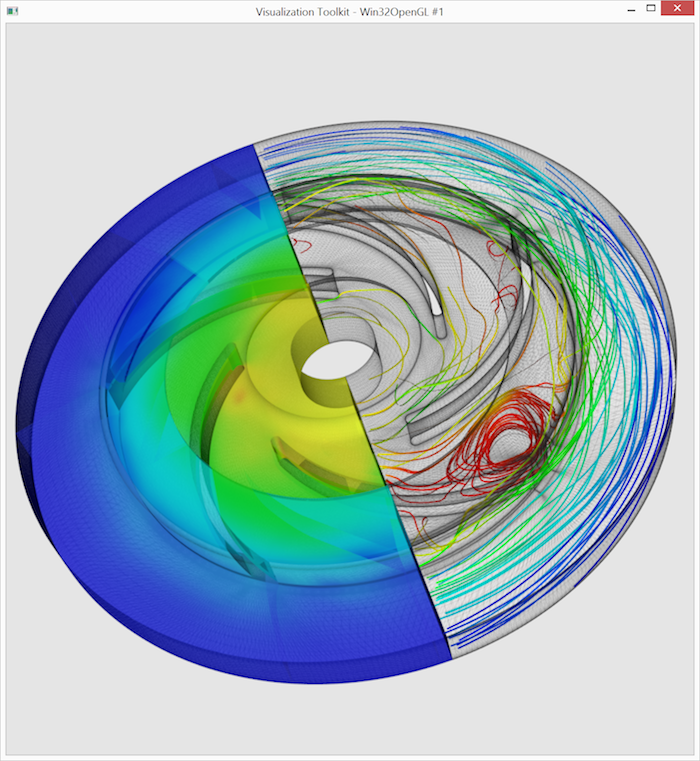
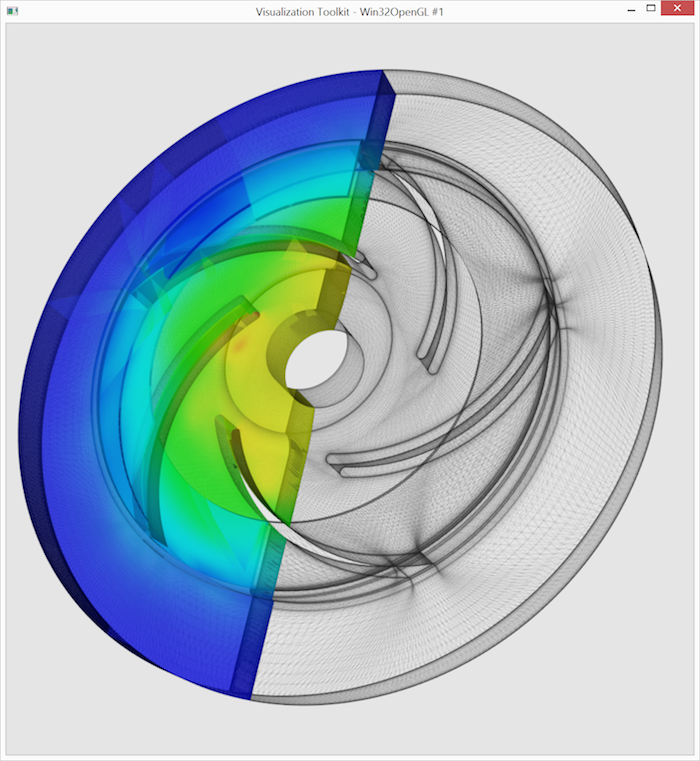
The Target

Our objective is to create the visualization depicted below using VTK. The dataset’s outline is shown as a semi-transparent wireframe for 3D context. The left portion displays pressure using color-coded surfaces (we’ll omit complex volume rendering here). To visualize the velocity field, the right portion is populated with streamlines, color-coded by velocity magnitude. This visualization choice, while not technically ideal, maintains code simplicity. The visualization challenge lies in the flow’s turbulence.

Step by Step

Let’s break down the VTK code, illustrating the rendering output at each stage. The complete source code is available for download at the end of this tutorial.

We begin by including necessary VTK components and defining the main function.

 1
 2
 3
 4
 5
 6
 7
 8
 9
10
11
12
13
14
15
16
17
18
19
20
21
22
23
24
25

#include <vtkActor.h>
#include <vtkArrayCalculator.h>
#include <vtkCamera.h>
#include <vtkClipDataSet.h>
#include <vtkCutter.h>
#include <vtkDataSetMapper.h>
#include <vtkInteractorStyleTrackballCamera.h>
#include <vtkLookupTable.h>
#include <vtkNew.h>
#include <vtkPlane.h>
#include <vtkPointData.h>
#include <vtkPointSource.h>
#include <vtkPolyDataMapper.h>
#include <vtkProperty.h>
#include <vtkRenderer.h>
#include <vtkRenderWindow.h>
#include <vtkRenderWindowInteractor.h>
#include <vtkRibbonFilter.h>
#include <vtkStreamTracer.h>
#include <vtkSmartPointer.h>
#include <vtkUnstructuredGrid.h>
#include <vtkXMLUnstructuredGridReader.h>

int main(int argc, char** argv)
{

Next, we set up the renderer and render window for displaying results, specifying the background color and render window size.

1
2
3
4
5
6
7
8
9

  // Setup the renderer
  vtkNew<vtkRenderer> renderer;
  renderer->SetBackground(0.9, 0.9, 0.9);

  // Setup the render window
  vtkNew<vtkRenderWindow> renWin;
  renWin->AddRenderer(renderer.Get());
  renWin->SetSize(500, 500);

This code would already display a static render window. However, we’ll incorporate vtkRenderWindowInteractor for interactive rotation, zooming, and panning.

1
2
3
4
5

  // Setup the render window interactor
  vtkNew<vtkRenderWindowInteractor> interact;
  vtkNew<vtkInteractorStyleTrackballCamera> style;
  interact->SetRenderWindow(renWin.Get());
  interact->SetInteractorStyle(style.Get());

Now, a running example with a blank gray render window appears.

We proceed to load the dataset using one of VTK’s numerous readers.

1
2
3

  // Read the file
  vtkSmartPointer<vtkXMLUnstructuredGridReader> pumpReader = vtkSmartPointer<vtkXMLUnstructuredGridReader>::New();
  pumpReader->SetFileName("rotor.vtu");

Brief overview of VTK memory management: VTK employs a user-friendly automatic memory management system based on reference counting. Unlike most implementations where the reference count resides within the smart pointer class, VTK stores it within the VTK objects themselves. This allows incrementing the reference count even when passing the VTK object as a raw pointer. Two primary methods exist for creating managed VTK objects: vtkNew<T> and vtkSmartPointer<T>::New(). The key difference is that vtkSmartPointer<T> can be implicitly cast to the raw pointer T* and returned from a function. For vtkNew<T> instances, we call .Get() to obtain a raw pointer and wrap it in a vtkSmartPointer for returning. This example doesn’t involve returning from functions, and all objects persist throughout; hence, we’ll primarily use the concise vtkNew, with the exception mentioned earlier for demonstration.

At this stage, the file remains unread. We or a downstream filter need to invoke Update() to trigger the reading process. While it’s generally best to let VTK classes manage updates, direct access to filter results (e.g., obtaining the pressure range in this dataset) necessitates manually calling Update(). (Multiple Update() calls don’t impact performance due to result caching.)

1
2
3
4

  // Get the pressure range
  pumpReader->Update();
  double pressureRange[2];
  pumpReader->GetOutput()->GetPointData()->GetArray("Pressure")->GetRange(pressureRange);

Next, we extract the dataset’s left half using vtkClipDataSet. We define a vtkPlane to mark the split and demonstrate VTK pipeline connections: successor->SetInputConnection(predecessor->GetOutputPort()). Requesting an update from clipperLeft ensures that all preceding filters are also updated through this connection.

1
2
3
4
5
6
7
8

  // Clip the left part from the input
  vtkNew<vtkPlane> planeLeft;
  planeLeft->SetOrigin(0.0, 0.0, 0.0);
  planeLeft->SetNormal(-1.0, 0.0, 0.0);

  vtkNew<vtkClipDataSet> clipperLeft;
  clipperLeft->SetInputConnection(pumpReader->GetOutputPort());
  clipperLeft->SetClipFunction(planeLeft.Get());

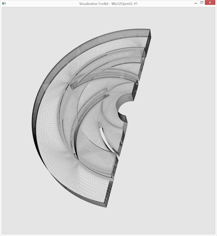
Finally, we create the first actors and mappers to display the left half’s wireframe rendering. Note that the mapper connects to its filter similarly to how filters connect to each other. The renderer typically triggers updates for all actors, mappers, and the underlying filter chains.

The line leftWireMapper->ScalarVisibilityOff(); might require clarification. It prevents pressure values (set as the active array) from coloring the wireframe.

 1
 2
 3
 4
 5
 6
 7
 8
 9
10
11
12

  // Create the wireframe representation for the left part
  vtkNew<vtkDataSetMapper> leftWireMapper;
  leftWireMapper->SetInputConnection(clipperLeft->GetOutputPort());
  leftWireMapper->ScalarVisibilityOff();

  vtkNew<vtkActor> leftWireActor;
  leftWireActor->SetMapper(leftWireMapper.Get());
  leftWireActor->GetProperty()->SetRepresentationToWireframe();
  leftWireActor->GetProperty()->SetColor(0.8, 0.8, 0.8);
  leftWireActor->GetProperty()->SetLineWidth(0.5);
  leftWireActor->GetProperty()->SetOpacity(0.8);
  renderer->AddActor(leftWireActor.Get());

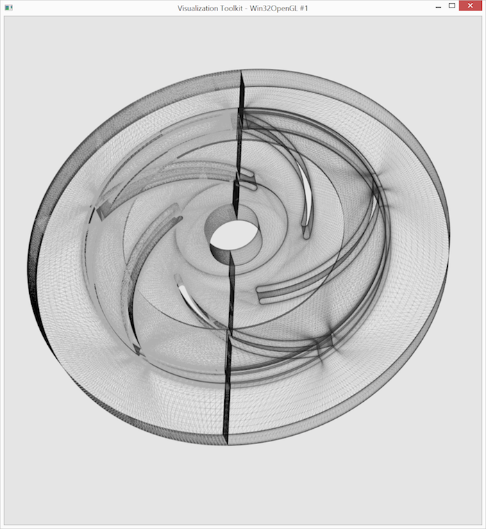
The render window now displays content: the left part’s wireframe.

Creating the right part’s wireframe follows a similar process. We reverse the plane normal of a new vtkClipDataSet, adjust the color and opacity of new mapper and actor instances, and observe the VTK pipeline branching into two directions (left and right) from the same input dataset.

 1
 2
 3
 4
 5
 6
 7
 8
 9
10
11
12
13
14
15
16
17
18
19
20
21

  // Clip the right part from the input
  vtkNew<vtkPlane> planeRight;
  planeRight->SetOrigin(0.0, 0.0, 0.0);
  planeRight->SetNormal(1.0, 0.0, 0.0);

  vtkNew<vtkClipDataSet> clipperRight;
  clipperRight->SetInputConnection(pumpReader->GetOutputPort());
  clipperRight->SetClipFunction(planeRight.Get());

  // Create the wireframe representation for the right part
  vtkNew<vtkDataSetMapper> rightWireMapper;
  rightWireMapper->SetInputConnection(clipperRight->GetOutputPort());
  rightWireMapper->ScalarVisibilityOff();

  vtkNew<vtkActor> rightWireActor;
  rightWireActor->SetMapper(rightWireMapper.Get());
  rightWireActor->GetProperty()->SetRepresentationToWireframe();
  rightWireActor->GetProperty()->SetColor(0.2, 0.2, 0.2);
  rightWireActor->GetProperty()->SetLineWidth(0.5);
  rightWireActor->GetProperty()->SetOpacity(0.1);
  renderer->AddActor(rightWireActor.Get());

As expected, the output window now presents both wireframe parts.

Let’s visualize some meaningful data. Adding pressure visualization to the left part is straightforward. We create a new mapper, connect it to clipperLeft, and enable coloring by the pressure array. Here, we utilize the previously derived pressureRange.

 1
 2
 3
 4
 5
 6
 7
 8
 9
10

  // Create the pressure representation for the left part
  vtkNew<vtkDataSetMapper> pressureColorMapper;
  pressureColorMapper->SetInputConnection(clipperLeft->GetOutputPort());
  pressureColorMapper->SelectColorArray("Pressure");
  pressureColorMapper->SetScalarRange(pressureRange);

  vtkNew<vtkActor> pressureColorActor;
  pressureColorActor->SetMapper(pressureColorMapper.Get());
  pressureColorActor->GetProperty()->SetOpacity(0.5);
  renderer->AddActor(pressureColorActor.Get());

The output resembles the image below. Low pressure in the center draws material into the pump, which is then transported outwards, experiencing a rapid pressure increase. (A color map legend with actual values would be ideal but is omitted for brevity.)

Now for the trickier part: drawing velocity streamlines in the right part. Streamlines are generated by integrating source points within a vector field, which is already present in the dataset as the “Velocities” vector array. We only need to generate the source points. vtkPointSource creates a sphere of random points. We’ll generate 1500 source points, knowing that most will fall outside the dataset and be ignored by the stream tracer.

1
2
3
4
5
6

  // Create the source points for the streamlines
  vtkNew<vtkPointSource> pointSource;
  pointSource->SetCenter(0.0, 0.0, 0.015);
  pointSource->SetRadius(0.2);
  pointSource->SetDistributionToUniform();
  pointSource->SetNumberOfPoints(1500);

We create the streamtracer and establish its input connections. You might wonder about “multiple” connections. This is our first encounter with a VTK filter accepting multiple inputs. The standard input connection receives the vector field, while the source connection receives the seed points. Since “Velocities” is the active vector array in clipperRight, explicit specification is unnecessary. We instruct the streamtracer to integrate in both directions from the seed points using the Runge-Kutta-4.5 integration method.

1
2
3
4
5

  vtkNew<vtkStreamTracer> tracer;
  tracer->SetInputConnection(clipperRight->GetOutputPort());
  tracer->SetSourceConnection(pointSource->GetOutputPort());
  tracer->SetIntegrationDirectionToBoth();
  tracer->SetIntegratorTypeToRungeKutta45();

The next challenge is coloring streamlines by velocity magnitude. As no array exists for this, we’ll calculate magnitudes into a new scalar array using the vtkArrayCalculator filter. This filter outputs the input dataset unchanged but adds a new array computed from existing ones. We configure it to calculate the “Velocity” vector’s magnitude and output it as “MagVelocity.” We manually call Update() again to determine the new array’s range.

 1
 2
 3
 4
 5
 6
 7
 8
 9
10

  // Compute the velocity magnitudes and create the ribbons
  vtkNew<vtkArrayCalculator> magCalc;
  magCalc->SetInputConnection(tracer->GetOutputPort());
  magCalc->AddVectorArrayName("Velocity");
  magCalc->SetResultArrayName("MagVelocity");
  magCalc->SetFunction("mag(Velocity)");

  magCalc->Update();
  double magVelocityRange[2];
  magCalc->GetOutput()->GetPointData()->GetArray("MagVelocity")->GetRange(magVelocityRange);

Since vtkStreamTracer directly outputs polylines, which vtkArrayCalculator passes through, we could display magCalc’s output directly using a new mapper and actor.

Instead, we’ll enhance the output by displaying ribbons. vtkRibbonFilter generates 2D cells to represent ribbons for all input polylines.

 1
 2
 3
 4
 5
 6
 7
 8
 9
10
11
12
13

  // Create and render the ribbons
  vtkNew<vtkRibbonFilter> ribbonFilter;
  ribbonFilter->SetInputConnection(magCalc->GetOutputPort());
  ribbonFilter->SetWidth(0.0005);

  vtkNew<vtkPolyDataMapper> streamlineMapper;
  streamlineMapper->SetInputConnection(ribbonFilter->GetOutputPort());
  streamlineMapper->SelectColorArray("MagVelocity");
  streamlineMapper->SetScalarRange(magVelocityRange);

  vtkNew<vtkActor> streamlineActor;
  streamlineActor->SetMapper(streamlineMapper.Get());
  renderer->AddActor(streamlineActor.Get());

The final step, also necessary for generating intermediate renderings, involves rendering the scene and initializing the interactor.

1
2
3
4
5
6

  // Render and show interactive window
  renWin->Render();
  interact->Initialize();
  interact->Start();
  return 0;
}

We arrive at the final visualization, presented again below:

The complete source code for this visualization is available here.

The Good, the Bad, and the Ugly

Let’s conclude with my personal pros and cons of the VTK framework.

• Pro: Active development: VTK benefits from active development by numerous contributors, primarily from academia. This ensures access to cutting-edge algorithms, support for various 3D formats, active bug fixing, and readily available solutions on discussion boards.

• Con: Reliability: Combining algorithms from different contributors with VTK’s open pipeline design can lead to issues with unusual filter combinations. I’ve delved into VTK’s source code to troubleshoot unexpected results in complex filter chains. Setting up VTK for debugging is highly recommended.

• Pro: Software Architecture: VTK’s pipeline design and overall architecture are well-conceived and enjoyable to work with. A few lines of code can produce remarkable results, and the built-in data structures are intuitive.

• Con: Micro Architecture: Some micro-architectural choices remain unclear. Const-correctness is practically nonexistent, and arrays are passed as inputs and outputs without clear distinction. I addressed this in my algorithms by sacrificing some performance and creating a vtkMath wrapper that utilizes custom 3D types like typedef std::array<double, 3> Pnt3d;.

• Pro: Micro Documentation: The Doxygen documentation for classes and filters is comprehensive and useful, while the wiki’s examples and test cases aid in understanding filter usage.

• Con: Macro Documentation: Although good VTK tutorials and introductions exist online, a comprehensive reference guide explaining specific tasks seems to be lacking. Expect to invest time in research when attempting something new. Finding the right filter for a task can also be challenging, but the Doxygen documentation usually suffices once you do. Experimenting with Paraview is a good way to explore VTK.

• Pro: Implicit Parallelization Support: Parallelization becomes simple if your sources can be divided into independently processed parts. This involves creating separate filter chains within each thread to handle a single part, which is common in large visualization problems.

• Con: No Explicit Parallelization Support: Utilizing multiple cores for non-divisible problems requires significant effort. You’ll need to determine thread-safe or re-entrant classes through trial-and-error or source code analysis. I once traced a parallelization issue to a VTK filter using a static global variable for a C library call.

• Pro: Buildsystem CMake: The cross-platform meta-build-system CMake, also developed by Kitware (VTK’s creator), is widely used. It integrates seamlessly with VTK, simplifying multi-platform build system setups.

• Pro: Platform Independence, License, and Longevity: VTK is inherently platform-independent and licensed under a very permissive BSD-style license. Professional support is available for critical projects. Backed by research institutions and companies, Kitware is likely to remain a prominent player.

Last Word

In conclusion, VTK is an exceptional data visualization tool for my preferred problem domain. If you encounter a project involving visualization, mesh processing, image processing, or similar tasks, consider exploring Paraview with an example input to assess VTK’s suitability for your needs.