TensorFlow, a leading deep learning tool developed by Google, excels at training and deploying complex neural networks. Its ability to optimize architectures with millions of parameters and its extensive toolkit for hardware acceleration, distributed training, and production workflows make it a powerful option. While these features might seem daunting for tasks outside deep learning, TensorFlow offers accessibility and usability for simpler problems as well. At its core, TensorFlow is an optimized library for tensor operations (vectors, matrices) and calculus operations for gradient descent on any sequence of calculations. Gradient descent, a cornerstone of computational mathematics, traditionally demanded application-specific code and equations. However, TensorFlow’s “automatic differentiation” architecture streamlines this process, as we will explore.

TensorFlow Applications

• Example 1: Linear Regression with Gradient Descent in TensorFlow 2.0

• Understanding Gradient Descent

• Example 2: Maximally Separated Unit Vectors

• Example 3: Creating Adversarial AI Inputs

• Concluding Thoughts: Gradient Descent Optimization

• TensorFlow’s Gradient Descent: From Minimums to AI System Attacks

Example 1: Linear Regression with Gradient Descent in TensorFlow 2.0

Example 1 Notebook

Before diving into the TensorFlow code, it’s crucial to grasp the concepts of gradient descent and linear regression.

Understanding Gradient Descent

In essence, gradient descent is a numerical method for determining the inputs to a system of equations that minimize its output. In the realm of machine learning, this system represents our model, the inputs are the unknown parameters, and the output is a loss function to be minimized, indicating the discrepancy between the model and the data. For certain problems, such as linear regression, equations exist to directly calculate the error-minimizing parameters. However, most practical applications necessitate numerical methods like gradient descent for a suitable solution.

The key takeaway here is that gradient descent typically involves defining equations and using calculus to derive the relationship between the loss function and parameters. TensorFlow, with its auto-differentiation capabilities, handles the calculus, allowing us to focus on solution design rather than implementation intricacies.

Let’s illustrate this with a simple linear regression problem. Given height (h) and weight (w) data for 150 adult males, we start with an initial estimate of the slope and standard deviation of the relationship. After around 15 iterations of gradient descent, we approach a near-optimal solution.

Let’s break down how this solution was achieved using TensorFlow 2.0.

In linear regression, we posit that weights can be predicted through a linear equation of heights.

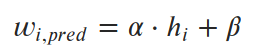
Our objective is to find the parameters α and β (slope and intercept) that minimize the average squared error (loss) between predicted and actual values. This loss function (mean squared error, or MSE) is represented as:

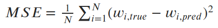
We can visualize the mean squared error for a couple of inaccurate lines and the exact solution (α=6.04, β=-230.5).

Now, let’s implement this using TensorFlow. The initial step is to code the loss function using tensors and tf.* functions.

1
2
3
4
5

def calc_mean_sq_error(heights, weights, slope, intercept):
    predicted_wgts = slope * heights + intercept
    errors = predicted_wgts - weights
    mse = tf.reduce_mean(errors**2)
    return mse

The code is quite straightforward. Standard algebraic operators work with tensors, so we ensure our variables are tensors and employ tf.* methods for other operations.

Next, we incorporate this into a gradient descent loop:

 1
 2
 3
 4
 5
 6
 7
 8
 9
10
11
12
13
14
15
16
17
18
19
20
21
22
23
24

def run_gradient_descent(heights, weights, init_slope, init_icept, learning_rate):
 
    # Any values to be part of gradient calcs need to be vars/tensors
    tf_slope = tf.Variable(init_slope, dtype='float32') 
    tf_icept = tf.Variable(init_icept, dtype='float32') 
    
    # Hardcoding 25 iterations of gradient descent
    for i in range(25):

        # Do all calculations under a "GradientTape" which tracks all gradients
        with tf.GradientTape() as tape:
            tape.watch((tf_slope, tf_icept))

            # This is the same mean-squared-error calculation as before
            predictions = tf_slope * heights + tf_icept
            errors = predictions - weights
            loss = tf.reduce_mean(errors**2)

        # Auto-diff magic!  Calcs gradients between loss calc and params
        dloss_dparams = tape.gradient(loss, [tf_slope, tf_icept])
       
        # Gradients point towards +loss, so subtract to "descend"
        tf_slope = tf_slope - learning_rate * dloss_dparams[0]
        tf_icept = tf_icept - learning_rate * dloss_dparams[1]

The elegance of this approach is noteworthy. Gradient descent involves calculating derivatives of the loss function with respect to all variables being optimized. While calculus is inherently involved, we didn’t explicitly perform any. The magic lies in:

1. TensorFlow constructing a computation graph of all calculations within a tf.GradientTape() scope.
2. TensorFlow’s ability to compute derivatives (gradients) for every operation, determining how variables within the graph affect each other.

How does this process behave with different starting points?

While gradient descent comes close to the optimal MSE, it converges to a significantly different slope and intercept compared to the true optimum in both scenarios. Sometimes, this is attributed to gradient descent settling into local minima. However, linear regression theoretically has a single global minimum. So, why did we arrive at an incorrect slope and intercept?

The issue lies in our simplification of the code for demonstration purposes. We omitted data normalization, and the slope parameter behaves differently from the intercept. Minute changes in slope can drastically impact the loss, while similar changes in intercept have minimal effect. This scale difference between trainable parameters leads to the slope dominating gradient calculations, rendering the intercept almost irrelevant.

Consequently, gradient descent primarily optimizes the slope near the initial intercept guess. Since the error is close to the optimum, the gradients are minuscule, resulting in tiny movements with each iteration. Data normalization would have mitigated this issue, but not completely eliminated it.

This example, though relatively simple, highlights how “auto-differentiation” handles complexity, as we’ll see in subsequent sections.

Example 2: Maximally Separated Unit Vectors

Example 2 Notebook

This example stems from an engaging deep learning exercise I encountered last year.

The premise involves a “variational auto-encoder” (VAE) capable of generating realistic faces from a set of 32 normally distributed numbers. For suspect identification, the goal is to utilize the VAE to produce a diverse set of (hypothetical) faces for witness selection, subsequently narrowing down the options based on similarity to chosen faces. While random initialization of vectors was suggested, I aimed for an optimal initial state.

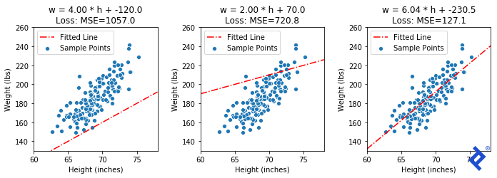
This can be framed as: Given a 32-dimensional space, find a set of X unit vectors that are maximally spread out. In two dimensions, the solution is straightforward. However, for higher dimensions (like 32), there’s no easy answer. But, by defining a suitable loss function minimized at our target state, gradient descent might provide a path.

Starting with a random set of 20 vectors (as depicted above), we’ll experiment with three increasingly complex loss functions to illustrate TensorFlow’s capabilities.

Let’s define our training loop, encapsulating the TensorFlow logic within the self.calc_loss() method. By overriding this method for each technique, we can reuse the loop.

 1
 2
 3
 4
 5
 6
 7
 8
 9
10
11
12
13
14
15
16
17
18
19

# Define the framework for trying different loss functions
# Base class implements loop, sub classes override self.calc_loss()
class VectorSpreadAlgorithm:
    # ...
    def calc_loss(self, tensor2d):
        raise NotImplementedError("Define this in your derived class")

    def one_iter(self, i, learning_rate):
        # self.vecs is an 20x2 tensor, representing twenty 2D vectors
        tfvecs = tf.convert_to_tensor(self.vecs, dtype=tf.float32)

        with tf.GradientTape() as tape:
            tape.watch(tfvecs)
            loss = self.calc_loss(tfvecs)

        # Here's the magic again. Derivative of spread with respect to
        # input vectors
        gradients = tape.gradient(loss, tfvecs)
        self.vecs = self.vecs - learning_rate * gradients

Our first technique is the simplest. We define a spread metric based on the angle between the two closest vectors. Since maximizing spread is our goal, we negate the metric for a minimization problem.

1
2
3
4
5
6
7
8
9

class VectorSpread_Maximize_Min_Angle(VectorSpreadAlgorithm):
    def calc_loss(self, tensor2d):
        angle_pairs = tf.acos(tensor2d @ tf.transpose(tensor2d))
        disable_diag = tf.eye(tensor2d.numpy().shape[0]) * 2 * np.pi
        spread_metric = tf.reduce_min(angle_pairs + disable_diag)    
        
        # Convention is to return a quantity to be minimized, but we want
        # to maximize spread. So return negative spread
        return -spread_metric

Matplotlib helps us visualize the results.

While rudimentary, it works. We update two vectors at a time, increasing their separation until they are no longer the closest, then shifting focus to the next closest pair. The key takeaway is that it works. TensorFlow successfully backpropagates gradients through tf.reduce_min() and tf.acos() to achieve the desired outcome.

Let’s introduce some complexity. Ideally, all vectors should have equal angles to their nearest neighbors at the optimal solution. So, we incorporate the “variance of minimum angles” into the loss function.

 1
 2
 3
 4
 5
 6
 7
 8
 9
10
11
12
13
14
15
16
17
18
19

class VectorSpread_MaxMinAngle_w_Variance(VectorSpreadAlgorithm):
    def spread_metric(self, tensor2d):
        """ Assumes all rows already normalized """
        angle_pairs = tf.acos(tensor2d @ tf.transpose(tensor2d))
        disable_diag = tf.eye(tensor2d.numpy().shape[0]) * 2 * np.pi
        all_mins = tf.reduce_min(angle_pairs + disable_diag, axis=1)    
        
        # Same calculation as before: find the min-min angle
        min_min = tf.reduce_min(all_mins)
        
        # But now also calculate the variance of the min angles vector
        avg_min = tf.reduce_mean(all_mins)
        var_min = tf.reduce_sum(tf.square(all_mins - avg_min))
        
        # Our spread metric now includes a term to minimize variance
        spread_metric = min_min - 0.4 * var_min

        # As before, want negative spread to keep it a minimization problem
        return -spread_metric

Now, the outlier vector quickly joins the cluster, as its large angle with its closest neighbor significantly increases the minimized variance. However, the globally-minimum angle still drives the process, albeit slowly. While improvements are possible in this 2D case, they might not generalize to higher dimensions.

The main point lies in the intricate tensor operations within the mean and variance calculations, and TensorFlow’s ability to track and differentiate each computation for every component in the input matrix without manual calculus.

Finally, let’s explore a force-based approach. Imagine each vector as a planet tethered to a central point, repelling each other. A physics simulation should lead us to our desired state.

My hypothesis is that gradient descent should also work. At the optimal solution, the net force on each planet from others should be zero (otherwise, they’d move). We can calculate the magnitude of force on each vector and use gradient descent to minimize it.

First, we define the force calculation method using tf.* methods:

 1
 2
 3
 4
 5
 6
 7
 8
 9
10
11
12
13
14
15
16
17

class VectorSpread_Force(VectorSpreadAlgorithm):
    
    def force_a_onto_b(self, vec_a, vec_b):
        # Calc force assuming vec_b is constrained to the unit sphere
        diff = vec_b - vec_a
        norm = tf.sqrt(tf.reduce_sum(diff**2))
        unit_force_dir = diff / norm
        force_magnitude = 1 / norm**2
        force_vec = unit_force_dir * force_magnitude

        # Project force onto this vec, calculate how much is radial
        b_dot_f = tf.tensordot(vec_b, force_vec, axes=1)
        b_dot_b = tf.tensordot(vec_b, vec_b, axes=1)
        radial_component =  (b_dot_f / b_dot_b) * vec_b

        # Subtract radial component and return result
        return force_vec - radial_component

Next, we define the loss function using the force function, accumulating the net force on each vector and calculating its magnitude. At the optimum, all forces should cancel out, resulting in zero net force.

 1
 2
 3
 4
 5
 6
 7
 8
 9
10
11
12
13
14
15
16
17
18
19
20
21
22
23
24
25
26
27
28

def calc_loss(self, tensor2d):
    n_vec = tensor2d.numpy().shape[0]
    all_force_list = []

    for this_idx in range(n_vec):

        # Accumulate force of all other vecs onto this one
        this_force_list = []
        for other_idx in range(n_vec):

            if this_idx == other_idx:
                continue

            this_vec = tensor2d[this_idx, :]
            other_vec = tensor2d[other_idx, :]

            tangent_force_vec = self.force_a_onto_b(other_vec, this_vec)
            this_force_list.append(tangent_force_vec)

        # Use list of all N-dimensional force vecs. Stack and sum.
        sum_tangent_forces = tf.reduce_sum(tf.stack(this_force_list))
        this_force_mag = tf.sqrt(tf.reduce_sum(sum_tangent_forces**2))

        # Accumulate all magnitudes, should all be zero at optimal solution
        all_force_list.append(this_force_mag)

    # We want to minimize total force sum, so simply stack, sum, return
    return tf.reduce_sum(tf.stack(all_force_list))

Not only does the solution work remarkably well (aside from initial chaos), but the credit goes to TensorFlow. It successfully traced gradients through numerous for loops, an if statement, and a complex web of calculations.

Example 3: Creating Adversarial AI Inputs

Example 3 Notebook

We begin by selecting an image classifier to target. Our choice is one of the top solutions from the Dogs vs. Cats Kaggle Competition, specifically, the solution by Kaggler “uysimty.” Kudos to them for the effective cat-vs-dog model and comprehensive documentation. This robust model boasts 13 million parameters across 18 neural network layers (further details in the corresponding notebook).

Note that our aim isn’t to expose flaws in this specific network, but rather to demonstrate the vulnerability of any standard neural network with numerous inputs.

After some adjustments, we successfully loaded the model and implemented the necessary image pre-processing.

The classifier appears quite reliable, with all sample classifications accurate and exceeding 95% confidence. Let’s attempt an attack!

Our objective is to create an image that’s clearly a cat but misclassified as a dog with high confidence. How do we achieve this?

Starting with a correctly classified cat image, we analyze how minute modifications in each color channel (values 0-255) of a pixel affect the classifier’s output. While tweaking one pixel might have a negligible impact, the cumulative effect of adjusting all 128x128x3 = 49,152 pixel values might yield the desired outcome.

But how do we determine the direction of these pixel adjustments? In standard neural network training, we minimize the loss between target and predicted labels, utilizing gradient descent in TensorFlow to update all 13 million parameters. Here, we’ll keep those parameters constant and instead adjust the input pixel values.

Our loss function? The “cat-ness” of the image! By calculating the derivative of the cat probability with respect to each pixel, we discover how to minimize the cat classification.

 1
 2
 3
 4
 5
 6
 7
 8
 9
10
11
12
13
14
15
16
17
18
19
20
21
22

def adversarial_modify(victim_img, to_dog=False, to_cat=False):
    # We only need four gradient descent steps
    for i in range(4):

        tf_victim_img = tf.convert_to_tensor(victim_img, dtype='float32')

        with tf.GradientTape() as tape:
            tape.watch(tf_victim_img)

            # Run the image through the model
            model_output = model(tf_victim_img)

            # Minimize cat confidence and maximize dog confidence 
            loss = (model_output[0] - model_output[1])

        dloss_dimg = tape.gradient(loss, tf_victim_img)

        # Ignore gradient magnitudes, only care about sign, +1/255 or -1/255
        pixels_w_pos_grad = tf.cast(dloss_dimg > 0.0, 'float32') / 255.
        pixels_w_neg_grad = tf.cast(dloss_dimg < 0.0, 'float32') / 255.

        victim_img = victim_img - pixels_w_pos_grad + pixels_w_neg_grad

Once again, Matplotlib aids in visualizing the results.

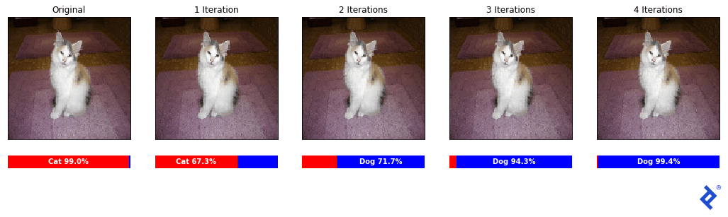
Remarkably, despite appearing identical to the human eye, the images after four iterations successfully fool the classifier into predicting a dog with 99.4% confidence!

Let’s confirm this isn’t a fluke by reversing the process.

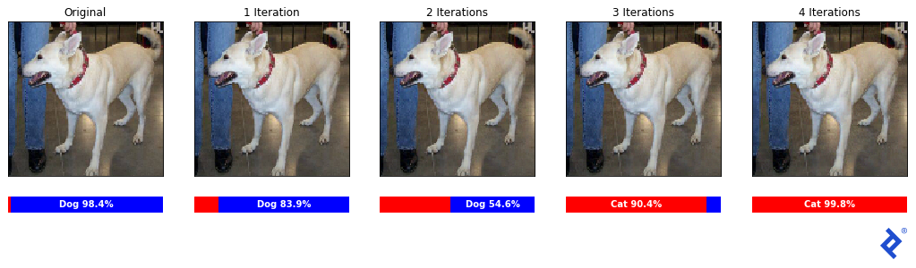
Success! The initially correctly classified dog (98.4% confidence) is now recognized as a cat with 99.8% confidence.

Finally, let’s examine the changes in a sample image patch.

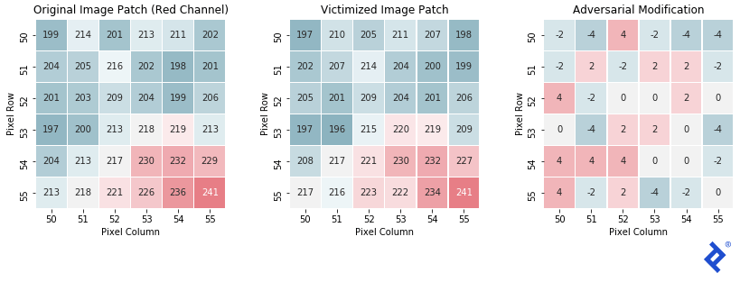
As anticipated, the final patch closely resembles the original, with each pixel’s red channel intensity shifting by -4 to +4. This subtle shift, imperceptible to humans, drastically alters the classifier’s output.

Concluding Thoughts: Gradient Descent Optimization

For simplicity, we manually applied gradients to trainable parameters. However, in practice, data scientists should leverage optimizers for their superior effectiveness.

Popular options include RMSprop, Adagrad, and Adadelta, with Adam being arguably the most prevalent. These “adaptive learning rate methods” dynamically adjust learning rates for each parameter, often incorporating momentum terms and approximating higher-order derivatives to escape local minima and accelerate convergence.

An animation from Sebastian Ruder illustrates various optimizers navigating a loss surface. Our manual techniques resemble “SGD,” highlighting the improved performance of advanced optimizers in most scenarios.

However, deep expertise in optimizers isn’t always necessary, even for those involved in artificial intelligence development services. Familiarization with a few key optimizers suffices to understand their role in enhancing TensorFlow’s gradient descent. In most cases, starting with Adam and experimenting with alternatives only when models struggle to converge is a pragmatic approach.

For those interested in the intricacies of optimizer functionality, Ruder’s overview (source of the animation) offers a comprehensive resource.

Let’s enhance our linear regression solution from earlier by incorporating optimizers. Here’s the original manual gradient descent code:

 1
 2
 3
 4
 5
 6
 7
 8
 9
10
11
12
13
14
15
16
17

# Manual gradient descent operations
def run_gradient_descent(heights, weights, init_slope, init_icept, learning_rate):
 
    tf_slope = tf.Variable(init_slope, dtype='float32') 
    tf_icept = tf.Variable(init_icept, dtype='float32') 
    
    for i in range(25):
        with tf.GradientTape() as tape:
            tape.watch((tf_slope, tf_icept))
            predictions = tf_slope * heights + tf_icept
            errors = predictions - weights
            loss = tf.reduce_mean(errors**2)

        gradients = tape.gradient(loss, [tf_slope, tf_icept])
        
        tf_slope = tf_slope - learning_rate * gradients[0]
        tf_icept = tf_icept - learning_rate * gradients[1]

Now, the same code using an optimizer (changes highlighted in blue):

 1
 2
 3
 4
 5
 6
 7
 8
 9
10
11
12
13
14
15
16
17
18
19
20
21
22
23
24
25

# Gradient descent with Optimizer (RMSprop)
    def run_gradient_descent(heights, weights, init_slope, init_icept, learning_rate):
     
        tf_slope = tf.Variable(init_slope, dtype='float32') 
        tf_icept = tf.Variable(init_icept, dtype='float32')
    
        # Group trainable parameters into a list
        trainable_params = [tf_slope, tf_icept]
    
        # Define your optimizer (RMSprop) outside of the training loop
        optimizer = keras.optimizers.RMSprop(learning_rate)
       
        for i in range(25):
            # GradientTape loop is the same
            with tf.GradientTape() as tape:
                tape.watch(trainable_params)
                predictions = tf_slope * heights + tf_icept
                errors = predictions - weights
                loss = tf.reduce_mean(errors**2)
    
            # We can use the trainable parameters list directly in gradient calcs
            gradients = tape.gradient(loss, trainable_params)
    
            # Optimizers always aim to *minimize* the loss function
            optimizer.apply_gradients(zip(gradients, trainable_params))

We define an RMSprop optimizer outside the loop and use optimizer.apply_gradients() after each gradient calculation to update parameters. The optimizer, residing outside the loop, tracks historical gradients for momentum and higher-order derivative calculations.

Let’s observe the outcome with the RMSprop optimizer.

Excellent! Now, let’s try the Adam optimizer.

Interestingly, Adam’s momentum mechanics cause it to overshoot and oscillate around the optimum. While beneficial for complex loss surfaces, it hinders us here. This emphasizes the importance of tuning the optimizer as a hyperparameter.

This pattern, widely used in custom TensorFlow architectures with complex loss functions, is crucial for deep learning practitioners. While our example involved only two parameters, it underscores the necessity of optimizers when dealing with millions.

TensorFlow’s Gradient Descent: From Minimums to AI System Attacks

All code snippets and images originate from notebooks in the corresponding GitHub repo, which also includes a summarized overview with links to individual notebooks for complete code access. For clarity, certain details were omitted but can be found in the inline documentation.

I hope this article provided valuable insights into leveraging gradient descent in TensorFlow. Even without direct application, it should offer a clearer understanding of modern neural network architectures: define a model, define a loss function, and employ gradient descent (often through optimizers) to fit the model to your data.

Toptal, a Google Cloud Partner, offers on-demand access to Google-certified experts for critical projects.