If you’re tired of feeling bored and are eager to tap into your creative side, building something visually stunning and artistic might be just the thing. Or perhaps you’re interested in learning to program and want to create something remarkable as quickly as possible. In either case, the Processing language is an excellent choice.
Of all the programming languages I’ve used, Processing stands out as one of the most enjoyable. It’s a straightforward language that’s easy to pick up, understand, and use, yet remarkably powerful. You can think of it as painting with code on a blank canvas. There are no strict rules or limitations to hinder your creativity—the only boundaries are those set by your imagination.

During my time in college, I worked as a teaching assistant for a program that introduced high school students to Processing. Many of them lacked a solid programming background, with some having never written a line of code. Amazingly, they were tasked with learning the language and building simple games in just five days. The program boasted a near-perfect success rate, with very few students struggling. In this article, we’ll be following a similar path. I’ve condensed the entire program into two parts. The first part will focus on the Processing language, providing a basic overview, a walkthrough, and some helpful tips and tricks. In the second part, we’ll dive into building a simple game step by step, explaining each stage in detail. To make our game accessible online, I’ll also demonstrate how to convert the code into JavaScript using p5.js.
Prerequisites
To easily understand and follow along with these articles, having a basic understanding of programming concepts is recommended. However, I won’t delve into advanced programming topics, so a surface-level understanding will suffice. While I’ll touch upon low-level ideas like object-oriented programming (OOP) in certain sections, these are not essential for grasping the core concepts and are included for curious readers interested in the structure of the language. Feel free to skip these parts if you prefer. Other than that, all you need is a desire to learn this fantastic language and the enthusiasm to create your own game!
How to Approach This Guide
I’m a firm believer in learning by doing and experimenting. The sooner you immerse yourself in creating your own game, the faster you’ll become comfortable with Processing. Therefore, my first suggestion is to actively try each step in your own coding environment. Processing offers a simple and user-friendly IDE (code editor) that you can download and install to follow along. You can download it from here.
Let’s get started!
Introducing the Processing Language
This section provides a concise technical overview of the language, covering its structure and offering insights into the compilation and execution process. It includes some advanced programming knowledge and touches on the Java environment. If you’d rather jump into coding and learn about the details later, feel free to skip to the “Fundamentals of Processing” section.
Processing is a visual programming language that allows you to express creative ideas through code. However, it’s not a standalone programming language in the strictest sense. Instead, it’s categorized as a “Java-esque” language, meaning it’s built upon the Java platform but with its own unique features. When you run your Processing code, it undergoes preprocessing and is converted directly into Java code. Java’s PApplet class serves as the foundation for all Processing sketches. To illustrate this, let’s examine a couple of basic Processing code blocks:
| |
These code blocks are transformed into something like this:
| |
As you can see, the Processing code block is encapsulated within a class that inherits from Java’s PApplet. Consequently, any classes you define within your Processing code are treated as inner classes.
The fact that Processing is built on Java offers several advantages, particularly for Java developers. Not only is the syntax familiar, but it also allows for actions like embedding Java code, libraries, and JAR files into sketches, seamlessly integrating Processing applets into Java applications, defining classes, and utilizing standard data types like int, float, char, and so on. You can even write Processing code directly within Eclipse with some initial setup. However, one thing you can’t do is incorporate AWT or Swing components into Processing sketches due to conflicts with Processing’s looping nature. Rest assured, we won’t be exploring any of those advanced techniques in this article.
Fundamentals of Processing
Processing code revolves around two primary parts: the setup and draw blocks. The setup block runs only once at the start of the program, while the draw block executes continuously. This continuous execution of the draw block is a fundamental concept in Processing. Anything you code within the draw block will run 60 times per second from top to bottom until the program is stopped. We’ll leverage this principle to build everything in our game. Whether it’s moving objects, updating scores, detecting collisions, implementing gravity, or handling other game logic—it all hinges on this refresh loop. Think of this loop as the heartbeat of our project. I’ll explain how to make the most of this heartbeat to breathe life into your code in later sections. For now, let’s get acquainted with the Processing IDE.
Getting to Know the Processing IDE

If you’ve made it this far without downloading the Processing IDE, now’s the perfect time to do it. Throughout this article, I’ll be presenting simple tasks for you to try out. Having the IDE up and running will allow you to practice these concepts firsthand. Here’s a brief introduction to the Processing IDE. It’s very intuitive and user-friendly, so we’ll keep this concise.
As you might expect, the run and stop buttons do exactly what their names imply. Clicking the run button compiles and executes your code. Processing programs are designed to run indefinitely until interrupted. You can terminate a program programmatically, but if you don’t, the stop button provides a manual way to do so.
The button resembling a butterfly to the right of the run and stop buttons is the debugger. While incredibly useful, the debugger warrants its own dedicated article, which is outside the scope of this one. For now, you can safely disregard it. The dropdown menu adjacent to the debugger button is where you can add or configure mods. Mods extend the functionality of Processing, enabling you to write code for Android, use Python, and more. Similar to the debugger, mods are beyond the scope of this article, so you can leave it set to the default Java mode.
The window within the code editor is where your sketches typically run. It’s currently empty in the image because we haven’t defined any properties like size, background color, or drawn anything yet.
The code editor itself is self-explanatory—it’s where you write your Processing code. One notable feature is the presence of line numbers (!) Older versions of Processing lacked this, and I can’t overstate how much of a welcome addition they were.
The black box below the code editor is the console. We’ll use it to display messages, which is particularly handy for debugging. The errors tab next to the console is where error messages will appear—another valuable feature introduced in Processing 3.0. In previous versions, errors were printed to the console, making them harder to track.
The Setup Block
As previously mentioned, the setup block is executed only once when the program starts. This makes it the ideal place for handling configurations and tasks you want to perform once, such as loading images or sounds. Let’s look at an example setup block. Go ahead and run this code in your own environment to see the results firsthand.
| |
We’ll cover styling methods like background(), fill(), and stroke() in the properties and settings sections. For now, focus on understanding how the settings and configurations within the setup block affect the entire sketch. Code in this block essentially establishes ground rules that apply throughout the program. Pay close attention to the following methods:
size() - This function, as the name suggests, configures the dimensions of your sketch. It must be the first line of code within the setup block. Here are the different ways to use it:
- size(width,height);
- size(width, height, renderer);
The width and height values are specified in pixels. The optional third parameter, renderer, determines the rendering engine used for your sketch. The default renderer is P2D. Available renderers include P2D (Processing 2D), P3D (Processing 3D, used for sketches involving 3D graphics), and PDF (for drawing 2D graphics directly into an Acrobat PDF file. More information can be found here). Both P2D and P3D renderers leverage OpenGL-compatible graphics hardware.
fullScreen() - Starting with Processing 3.0, the fullScreen function provides an alternative to the size() function. Like size(), it should also be the first line within the setup block. Here’s how to use it:
- fullScreen();
- fullScreen(display);
- fullScreen(renderer);
- fullScreen(display, renderer);
Using it without any parameters runs your Processing sketch in fullscreen mode on your primary display. The ‘display’ parameter lets you specify which display to use for your sketch, which is useful when you have external monitors connected. For instance, setting ‘display’ to 2 (or 3, 4, etc.) will run the sketch on your second monitor. The ‘renderer’ parameter functions the same way as described for the size() function.
The Settings Block
The settings block is another new addition in recent Processing releases. Like setup and draw, it’s a code block that proves useful when you need to define methods like size() or fullScreen() using variable parameters. It’s also necessary for defining size() and other styling properties, such as smooth(), when working outside of the Processing IDE, such as in Eclipse. However, in most cases, and certainly for the content of this article, you won’t be needing it.
The Draw Block
There’s nothing inherently remarkable about the draw block itself, and yet it’s where all the excitement unfolds. Consider it the heart of your program, tirelessly beating 60 times per second. This block houses the core logic of your code, including all the shapes, objects, and interactions that bring your creation to life.
A significant portion of the code we’ll discuss will reside within the draw block. Understanding how it functions is crucial. To demonstrate, let’s try something. First, it’s important to know that you can print messages to the console using the print() or println() methods. While both print to the console, println appends a newline character at the end, resulting in each println() output appearing on a separate line.
Now, let’s examine the following code block. Before running it, try to predict what it will print to the console.
| |
If you guessed “1 1 1 1…”, you’re spot on! This often trips up people new to Processing. Remember that this block continuously loops. Each time it runs, x is reset to 0, incremented by 1, and printed to the console. This is why we get “1 1 1…” instead of “1 2 3…”. While somewhat obvious in this example, this behavior can lead to confusion in more complex scenarios.
To prevent x from being overwritten and achieve the desired “1 2 3…” output, we can utilize global variables. It’s a simple concept—we define the variable outside the draw block so its value persists across iterations. This also makes the variable accessible throughout the entire sketch. Take a look at the modified code:
| |
You might wonder how a variable defined outside our blocks can work and why we didn’t use the setup() block for this purpose since it executes only once at the beginning. The answer lies in the realm of object-oriented programming and scopes. If you’re unfamiliar with these concepts, feel free to skip this paragraph. Recall how Processing code gets converted into Java and wrapped within a Java class. The variables we define outside of setup() and draw() are treated as fields of this outer class. Using x += 1 in this context is equivalent to using this.x += 1. Since there’s no local variable named x within the draw() block’s scope, it searches outward and finds this.x. Why not define x within setup()? Doing so would limit the scope of x to the setup() function, making it inaccessible from the draw() block.
Drawing Shapes and Text
Now that we’re comfortable configuring our sketch with the setup block and understand how the draw block operates, let’s move on to the visually engaging aspects of Processing: drawing shapes.
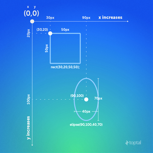
Before we proceed, it’s essential to grasp the concept of the coordinate system. In Processing, you specify the position of everything you draw on the screen using coordinates measured in pixels. The origin (0, 0) is located at the top-left corner, and all coordinates are relative to this point. Keep in mind that different shapes have different reference points. For instance, the reference point for rect() is its top-left corner, while for ellipse(), it’s the center. You can change these reference points using methods like rectMode() and ellipseMode(), which we’ll discuss in the properties and settings section. Refer to the accompanying figure for a visual representation.
This article provides a foundational overview of Processing, so we won’t delve into complex shapes like vertexes or 3D shapes. Rest assured, basic 2D shapes are more than sufficient for creating our game. The figure illustrates how to draw various shapes. Each shape has its syntax, but the underlying principle is to provide either its coordinates, its dimensions, or both. Familiarize yourself with the following commonly used shapes:
point() - Draws a single point at the specified coordinates. Usage:
- point(x, y)
- point(x, y, z) - For 3D sketches.
line() - Creates a line between two points. Usage:
- line(x1, y1, x2, y2)
- line(x1, y1, z1, x2, y2, z2) - For 3D sketches.
triangle() - Draws a triangle. Usage: triangle(x1, y1, x2, y2, x3, y3)
quad() - Draws a quadrilateral. Usage: quad(x1, y1, x2, y2, x3, y3, x4, y4)
rect() - Creates a rectangle. The reference point is the top-left corner by default (see figure). Usage:
- rect(x, y, w, h)
- rect(x, y, w, h, r) - ‘r’ specifies the corner radius in pixels for rounded corners.
- rect(x, y, w, h, tl, tr, br, bl) - Allows you to set individual radii for the top-left (tl), top-right (tr), bottom-right (br), and bottom-left (bl) corners, all in pixels.
ellipse() - Draws an ellipse. You can create a circle by specifying the same width and height values. The reference point is the center by default (see figure). Usage:
- ellipse(x, y, w, h)
arc() - Draws an arc. Usage:
- arc(x, y, w, h, start, stop) - ‘start’ and ‘stop’ define the starting and ending angles of the arc in radians. You can use constants like “PI, HALF_PI, QUARTER_PI and TWO_PI.”
- arc(x, y, w, h, start, stop, mode) - ‘mode’ determines the rendering style of the arc (string). Options include “OPEN, CHORD, PIE.” OPEN leaves the non-drawn portions without a border, CHORD completes them with a border, and PIE creates a pie chart-like appearance.
Displaying text on the screen is conceptually similar to drawing shapes—you provide coordinates where you want the text to appear. However, text handling offers more control, which we’ll explore in the properties and settings section. For now, let’s cover the basics.
text() - Displays text. Usage:
- text(c, x, y) - ‘c’ represents a single character.
- text(c, x, y, z) - For 3D sketches.
- text(str, x, y) - ‘str’ is the string to display.
- text(str, x, y, z) - For 3D sketches.
- text(num, x, y) - ’num’ is a numeric value.
- text(num, x, y, z) - For 3D sketches.
Working with Properties and Settings
Let’s start by understanding how setting object properties works. Properties encompass attributes like fill color, background color, border width, border color, shape alignment, border styles, and more.
The key is to remember that code execution flows from top to bottom. For example, if you set the “fill” property to red, all objects drawn after that line will be filled with red until another fill property overrides it. This behavior applies to other properties as well, although not all properties overwrite each other. For instance, the “stroke” property doesn’t replace the “fill” property; instead, they work in tandem. The image below illustrates this logic:
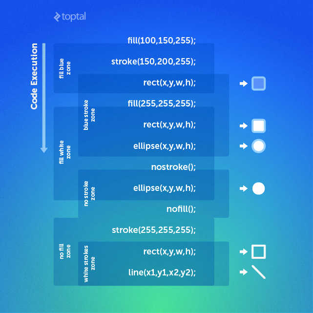
In the image, the first line sets the fill color to red, followed by the stroke color being set to blue. This establishes two active settings: red fill and blue stroke. As a result, the object drawn on the next line, regardless of its type, will have a red fill and a blue stroke (if applicable). Continue analyzing the image in this manner, and the underlying logic will become clear.
Here are some essential properties and settings you’ll frequently use:
Styling Settings
fill() - Sets the fill color for objects, including text. For now, we’ll focus on this usage:
- fill(r, g, b) - Red, green, and blue values as integers.
- fill(r, g, b, a) - Adds an alpha value for transparency, with a maximum of 255.
noFill() - Makes the fill color transparent.
stroke() - Sets the stroke color for objects, applicable to lines and object borders. Usage:
- stroke(r, g, b) - Red, green, and blue values as integers.
- stroke(r, g, b, a) - Adds an alpha value (max 255).
noStroke() - Removes the stroke.
strokeWeight() - Sets the stroke width. Usage:
- strokeWeight(x) - ‘x’ is an integer representing the stroke width in pixels.
background() - Sets the background color. Usage:
- background(r, g, b) - Red, green, and blue values.
- background(r, g, b, a) - Includes an alpha value (max 255).
Alignment Settings
ellipseMode() - Controls the reference point for aligning ellipses. Usage:
- ellipseMode(mode) - ‘mode’ specifies the alignment mode. Options include:
- CENTER (default): Center of the ellipse.
- RADIUS: Also uses the center, but the width and height values are treated as radii.
- CORNER: Uses the top-left corner.
- CORNERS: The first two parameters (x, y) define the top-left corner, and the last two (w, h) define the bottom-right corner. Width and height are irrelevant in this mode. Think of it as ellipse(x_tl, y_tl, x_br, y_br).
rectMode() - Similar to ellipseMode(), it sets the reference point for aligning rectangles. Usage:
- rectMode(mode) - ‘mode’ options:
- CENTER: Center of the rectangle.
- RADIUS: Center, but width and height are treated as half the width and height.
- CORNER (default): Top-left corner.
- CORNERS: First two parameters (x, y) for the top-left corner, last two (w, h) for the bottom-right corner. In this mode, width and height are disregarded. It’s best understood as rect(x_tl, y_tl, x_br, y_br).
Text-Related Settings
textSize() - Sets the font size of text. Usage:
- textSize(size) - Integer value representing the desired font size.
textLeading() - Controls the line height for text. Usage:
- textLeading(lineheight) - Pixel value specifying the space between lines.
textAlign() - Sets the reference point for aligning text. Usage:
- textAlign(alignX) - ‘alignX’ for horizontal alignment: LEFT, CENTER, RIGHT.
- textAlign(alignX, alignY) - ‘alignY’ for vertical alignment: TOP, BOTTOM, CENTER, BASELINE.
Bringing Objects to Life with Animation
We’ve covered drawing shapes and text, but they’re currently static. Let’s introduce movement! The concept is straightforward: instead of using fixed integer values for coordinates, we’ll use variables that we can increment or decrement. Consider this code:
| |
Notice how we achieve animation. We declare x and y as global variables, initializing them to 0. Within the draw loop, we create our ellipse, set its fill color to red, stroke color to blue, and use x and y for its coordinates. By incrementing x and y, we make the ball move. However, there’s a subtle issue with this code. Can you spot it? As a quick challenge, try to identify the problem and test it out. Here’s the result:

This behavior highlights the looping nature of Processing. Remember the “Draw Block” example and why we got “1 1 1…” instead of “1 2 3…”? The same principle applies here. Each time the draw block runs, x and y are incremented, causing the ball to redraw at a new location. However, the previously drawn balls remain visible. How can we make them disappear?
The solution is to move the background(255) line from the setup block to the very beginning of the draw block. When it was in setup, it executed only once, setting the background to white. We need it to repaint the background white in each loop iteration to cover the balls drawn in previous frames. By placing it as the first line in draw, it acts as the base layer. In each loop, the canvas is first cleared to white, and then new elements are drawn on top.
This illustrates the fundamental idea behind animation in Processing—programmatically manipulating object coordinates to create movement. But how do we implement more sophisticated behavior, such as confining the ball within the screen or simulating gravity? We’ll explore these concepts through hands-on exercises in the next part of this article. By the end, you’ll have created a fully functional, playable, and hopefully entertaining game!
Interacting with the Keyboard and Mouse
Processing simplifies keyboard and mouse interactions. Dedicated methods are triggered for each event, and the code within these methods executes when the event occurs. Additionally, you can utilize global variables like mousePressed and keyPressed within the draw block to leverage the loop. Let’s examine some of these methods:
| |
As you can see, checking for mouse clicks or specific key presses is incredibly straightforward. The mousePressed and keyCode variables provide additional options. mousePressed supports LEFT, RIGHT, and CENTER, while keyCode offers a wider range, including UP, DOWN, LEFT, RIGHT, ALT, CONTROL, SHIFT, BACKSPACE, TAB, ENTER, RETURN, ESC, and DELETE.
One crucial aspect, especially for our game, is obtaining the mouse coordinates. Processing provides the mouseX and mouseY variables for this purpose. You can directly use them within the draw() block to get the real-time position of the mouse cursor. For a comprehensive list of available methods and variables, refer to the Processing Reference.
Wrapping Up
By now, you should have a solid grasp of Processing’s fundamentals. However, knowledge without practice tends to fade quickly. I highly recommend continuing to experiment with what you’ve learned. To solidify your understanding, I’ve prepared two exercises. Challenge yourself to complete them independently. If you find yourself stuck, remember that Google and Processing Reference are your best resources. While I’ll provide the code for the first exercise, avoid looking at it until you’ve given it your best shot.
Exercise 1
Create four balls of different colors starting at the four corners of the screen. Make them travel towards the center at different speeds. When the mouse button is clicked and held, the balls should freeze. Upon releasing the mouse button, they should return to their initial positions and resume movement. Strive for something similar to this.
After attempting this exercise, you can find the code solution here.
Exercise 2
Remember the classic DVD screensaver screensaver where the DVD logo bounced around, and everyone eagerly anticipated it hitting the corner? Recreate this screensaver but with a rectangle instead of the logo. The screen should be black initially, and the rectangle should start at a random position. Each time it hits a corner, it should change color and reverse direction. Additionally, when you move the mouse, the rectangle should vanish, and the background should turn white (it is a screensaver, after all!). I won’t provide the code for this exercise here. Challenge yourself to implement it, and the code will be revealed in the second part of this article.
Stay tuned for the second part of the ultimate guide to Processing, where we’ll walk through building a simple game step by step.