Handling non-numerical data can be challenging, even for seasoned data scientists. Machine learning models typically require numerical features, not words, emails, websites, lists, graphs, or probability distributions. Transforming such data into a vector space is crucial, but how?
One common method is to represent non-numerical features as categorical. This works well if the category count is limited (like professions or countries). However, applying this to emails, for instance, would result in as many categories as samples, rendering the approach ineffective.
Alternatively, we can establish a distance metric between data points, quantifying their proximity. Similarly, a similarity measure provides the same information inversely—closer samples have higher similarity. Calculating distances (or similarities) for all data pairs yields a distance (or similarity) matrix, which provides usable numerical data.
However, this matrix’s dimensionality equals the sample count, posing challenges for feature usage (see curse of dimensionality) or visualization (while one plot can handle even 6D, visualizing a 100D plot is rare). Can we reduce dimensions while retaining crucial information?
The answer is yes, using embeddings.
What Is an Embedding and Why Use It?
An embedding is a compact, lower-dimensional representation of high-dimensional data. While not capturing all information, a good embedding retains enough to solve the task at hand.
Many embeddings are tailored for specific data types, like word2vec](https://en.wikipedia.org/wiki/Word2vec) for text or Fourier descriptors for shape images. However, we’ll focus on applying embeddings to any data with a defined distance or similarity measure. As long as we can calculate a distance matrix, the data’s nature—emails, lists, [trees, web pages—becomes irrelevant.
This article explores various embedding types, their workings, and applications in solving real-world problems with complex data. We’ll also cover their pros, cons, and alternatives, acknowledging that no single solution fits all machine learning challenges.
Let’s begin.
How Embeddings Work
All embeddings aim to reduce data dimensionality while preserving crucial information, each with its own approach. Here, we’ll examine a few popular ones applicable to distance or similarity matrices.
We won’t cover every embedding—there are dozens of well-known ones and countless lesser-known variations, each with its strengths and weaknesses.
For further exploration, consider these resources:
Distance Matrix
Choosing a suitable distance metric requires problem understanding, mathematical intuition, and sometimes, a bit of luck. In our approach, this choice significantly impacts the project’s success.
Remember these technical aspects: Many algorithms assume a distance (or dissimilarity) matrix $\textbf{D}$ with zeros on the diagonal and symmetry. If not symmetric, use $(\textbf{D} + \textbf{D}^T) / 2$. Algorithms using the kernel trick also assume distance as a metric, satisfying the triangle inequality:
[\forall a, b, c ;; d(a,c) \leq d(a,b) + d(b,c)]
To convert a distance matrix to a similarity matrix (if required), apply a monotone-decreasing function, like $\exp -x$.
Principal Component Analysis (PCA)
Principal Component Analysis, or PCA, is arguably the most common embedding technique. Its principle is simple: Find a linear feature transformation that maximizes captured variance, equivalently minimizing quadratic reconstruction error.
Let $\textbf{X} \in \mathbb{R}^{n \times p}$ be a sample matrix with $n$ features and $p$ dimensions, assuming zero sample mean for simplicity. We can reduce dimensions from $p$ to $q$ by multiplying $\textbf{X}$ with an orthonormal matrix $\textbf{V}_q \in \mathbb{R}^{p \times q}$:
[\hat{\textbf{X}} = \textbf{X} \textbf{V}_q]
This gives us $\hat{\textbf{X}} \in \mathbb{R}^{n \times q}$, the new feature set. Reconstruction, mapping back to the original space, involves multiplying by $\textbf{V}_q^T$.
We seek $\textbf{V}_q$ minimizing the reconstruction error:
[\min_{\textbf{V}_q} ||\textbf{X}\textbf{V}_q\textbf{V}_q^T - \textbf{X}||^2]
Columns of $\textbf{V}_q$ are principal component directions, and columns of $\hat{\textbf{X}}$ are principal components. $\textbf{V}_q$ can be found using SVD-decomposition of $\textbf{X}$, among other methods.
PCA applies directly to numerical features or distance/similarity matrices for non-numerical data.
In Python, PCA is implemented in implemented in scikit-learn.
Advantage: Fast computation and robustness to noise.
Disadvantage: Captures only linear structures, potentially losing non-linear information.
Kernel PCA
Kernel PCA is a non-linear extension of PCA, employing the kernel trick familiar from Support Vector Machines (SVM).
One way to compute PCA is through eigendecomposition of the double-centered gram matrix $\textbf{X} \textbf{X}^T \in \mathbb{R}^{n \times n}$. Kernel PCA computes a kernel matrix $\textbf{K} \in \mathbb{R}^{n \times n}$ and treats it as a gram matrix to find principal components.
Given feature samples $x_i$, $i \in {1,..,n}$, the kernel matrix is defined by a kernel function $K(x_i,x_j)=\langle \phi(x_i),\phi(x_j) \rangle$.
A common choice is the radial kernel:
[K(x_i,x_j)=\exp -\gamma \cdot d(x_i,x_j)]
where $d$ is the distance function.
Kernel PCA requires specifying a distance. For numerical features, Euclidean distance is suitable: $d(x_i,x_j)=\vert\vert x_i-x_j \vert \vert ^2$. Non-numerical features may require more creative distance definitions, keeping in mind the metric assumption.
Python’s implementation of Kernel PCA is in implemented in scikit-learn.
Advantage: Captures non-linear data structures.
Disadvantage: Sensitive to noise and heavily influenced by the choice of distance and kernel functions.
Multidimensional Scaling (MDS)
Multidimensional scaling (MDS) focuses on preserving global pairwise distances between samples. This intuitive idea works effectively with distance matrices.
Given feature samples $x_i$, $i \in {1,..,n}$, and distance function $d$, MDS finds new features $z_i \in \mathbb{R}^{q}$, $i \in {1,..,n}$, minimizing a stress function:
[\min_{z_1,..,z_n} \sum_{1 \leq i < j \leq n} (d(x_i, x_j) - ||z_i - z_j||)^2]
In Python, MDS is available in implemented in scikit-learn. However, scikit-learn does not support transformation of out-of-sample points, limiting its use with regression or classification models. In principle, though, it is possible.
Advantage: Aligns well with our framework and is robust to noise.
Disadvantage: Scikit-learn’s implementation is slow and lacks out-of-sample transformation support.
Use Case: Shipment Tracking
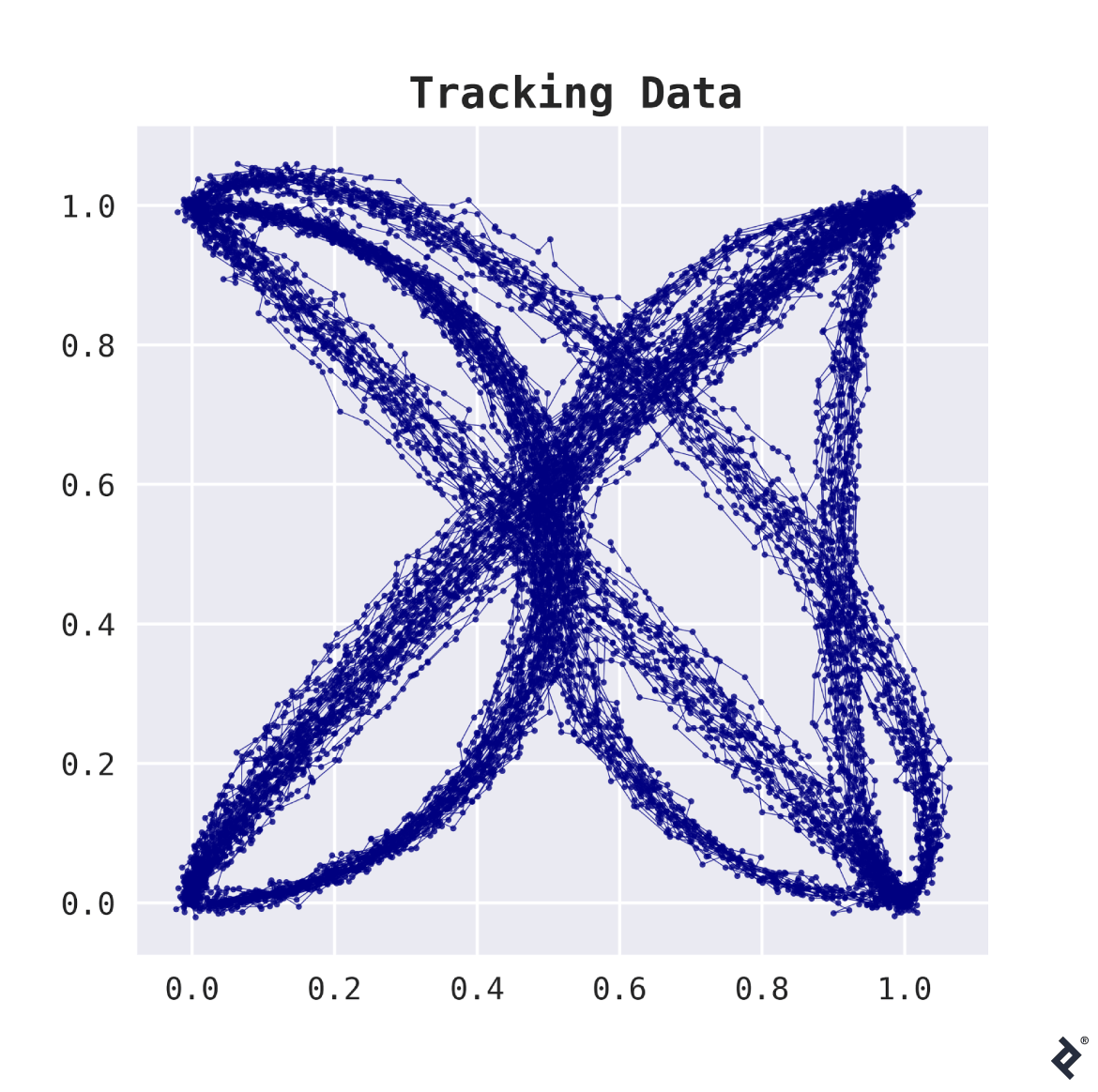
On a small tropical island, several settlements have established parcel delivery services for the local tourism industry. One merchant, seeking a competitive advantage, implements a satellite tracking system for all packages shipped on the island. With data in hand, the merchant calls upon a data scientist (that’s us!) to answer a crucial question: Can we predict a package’s destination while it’s en route?
The dataset contains 200 tracked shipments. For each shipment, a list of (x,y)-coordinates indicates locations where the package was detected, typically 20 to 50 observations per shipment. The plot below illustrates this data.
This data presents two key challenges.
First, its high dimensionality—with 50 locations per package, we have 100 dimensions, a significant number compared to the 200 samples.
Second, different routes have varying observation counts, hindering tabular representation by simply stacking coordinate lists.
The merchant anxiously taps the table, while the data scientist tries to remain composed.
This is where distance matrices and embeddings come to the rescue. We need a way to compare shipment routes. Fréchet distance seems suitable. With a distance defined, we can construct a distance matrix.
Note: This step can be computationally intensive. We need to compute $O(n^2)$ distances, each requiring $O(k^2)$ iterations, where $n$ is the sample count and $k$ is the observation count per sample. Efficient distance function implementation is crucial. In Python, tools like numba can significantly speed up this process.
Visualizing Embeddings
Now, we can employ an embedding to reduce the dimensionality from 200 to a manageable number. Given the limited trade routes, we can expect a reasonable representation in two or three dimensions. We’ll utilize PCA, Kernel PCA, and MDS for this purpose.
The plots below show labeled route data (for demonstration) and their 2D and 3D embedding representations (left to right). The labeled data depicts four trading posts connected by six trade routes, two of which are bidirectional, resulting in eight shipment groups (6+2). Notice the clear separation of all eight groups in the 3D embeddings.
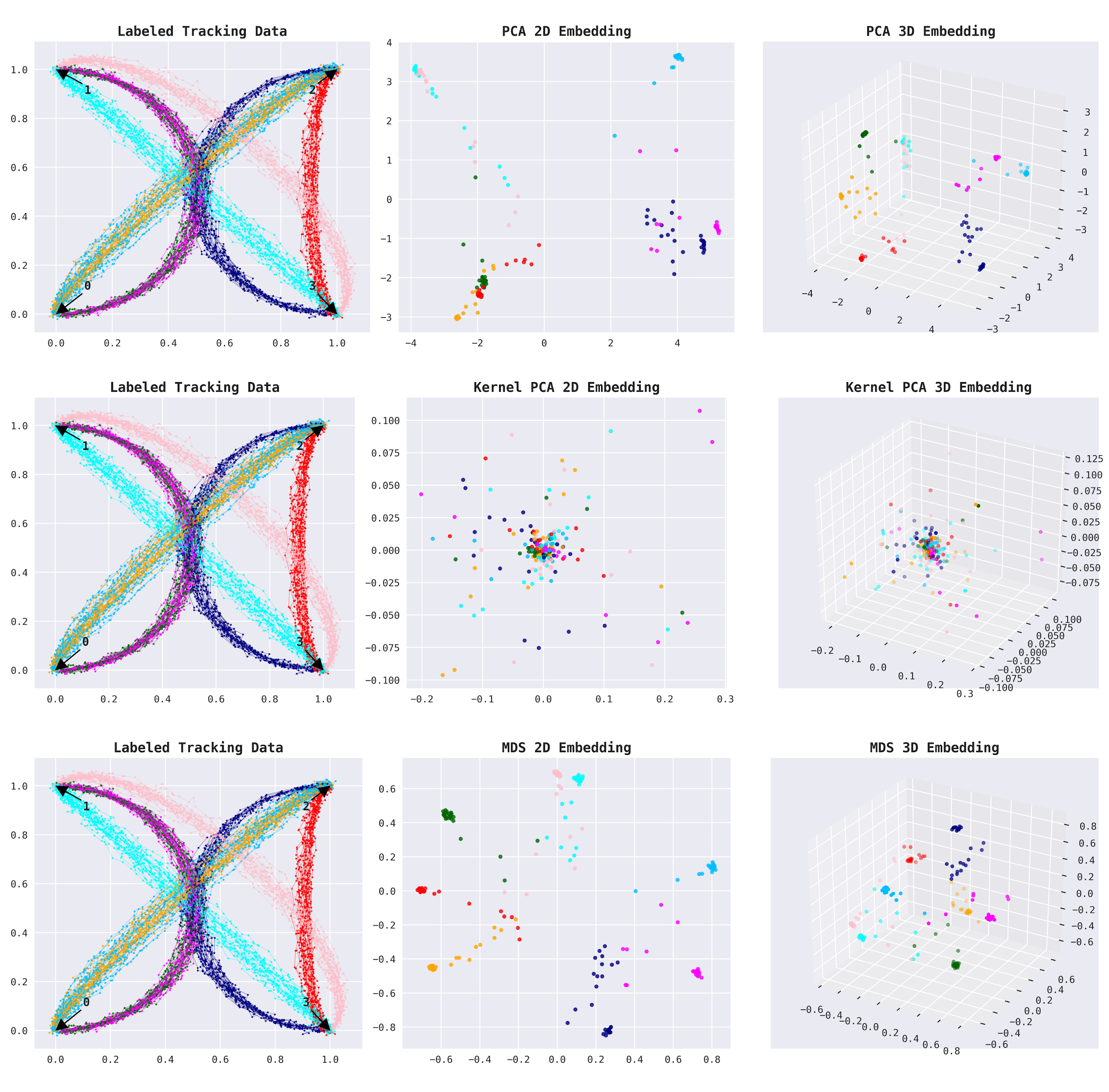
This is a promising start.
Embeddings in a Model Pipeline
We’re ready to train an embedding. While MDS performed well, its slow speed and lack of out-of-sample transformation support in scikit-learn make it less ideal for production. We’ll opt for Kernel PCA instead, remembering to apply a radial kernel to the distance matrix beforehand.
How do we choose the output dimension count? Analysis suggests 3D is sufficient, but to be safe and retain important information, we’ll set it to 10D. For optimal performance, treat the output dimension count as a hyper-parameter and tune it via cross-validation.
This gives us 10 numerical features suitable as input for various classification models. Let’s test Logistic Regression and Gradient Boosting, along with these models using the full distance matrix as input. Additionally, we’ll include SVM, which is designed for distance matrices directly.
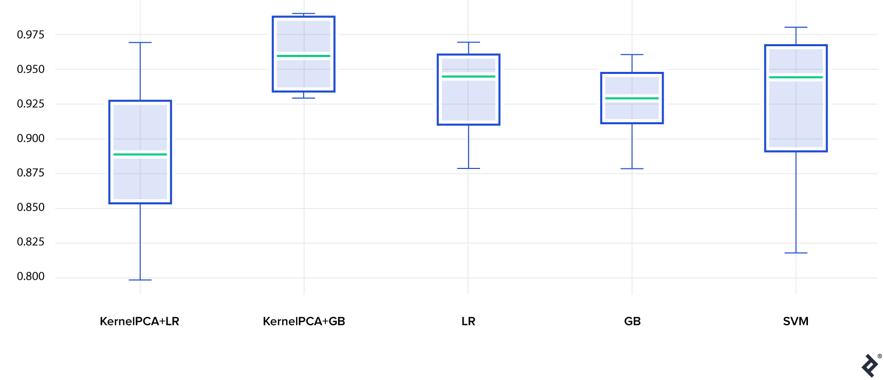
The table below shows model accuracies on the test set (using 10 train-test splits to estimate variance):
- Gradient Boosting with an embedding (KernelPCA+GB) achieves the highest accuracy, outperforming Gradient Boosting without an embedding (GB), highlighting Kernel PCA’s benefit.
- Logistic Regression performs reasonably well. Interestingly, Logistic Regression without an embedding (LR) performs better than with an embedding (KernelPCA+LR). This is not entirely surprising, as linear models are less flexible but less prone to overfitting. Here, information loss from the embedding seems to outweigh the advantage of reduced input dimensionality.
- Finally, SVM performs well, although with higher variance.
Model Accuracy
The Python code for this use case is available is available at GitHub.
Conclusion
We’ve explored embeddings and their use with distance matrices for solving real-world problems. Now, let’s assess their overall value.
Pros & Cons of Using Embeddings
Pros:
Enables working with uncommon or complex data by defining a distance metric, often achievable with knowledge, creativity, and a touch of luck.
Produces low-dimensional numerical data suitable for analysis, clustering, or as features for various machine learning models.
Cons:
Involves information loss during:
- Replacing original data with a similarity matrix
- Dimensionality reduction through embedding
Distance matrix computation can be time-consuming depending on the data and distance function, requiring efficient implementation.
Susceptibility to noise, mitigated by careful data cleaning.
Sensitivity to hyper-parameter choices, requiring analysis or tuning.
Alternatives: Why Not Use…?
Why not embed data directly instead of using a distance matrix? If a suitable embedding for direct encoding exists, use it. However, this is not always guaranteed.
Why not cluster data based on the distance matrix? This is valid for dataset segmentation. Some clustering methods, like Spectral Clustering](https://scikit-learn.org/stable/modules/clustering.html#spectral-clustering), utilize embeddings. For further exploration, refer to this [clusterization tutorial.
Why not use the distance matrix directly as features? Distance matrices have dimensions of $(n_{samples}, n_{samples})$. Not all models handle this efficiently—some overfit, some are slow, and some fail entirely. Models with low variance, like linear or regularized models, are better suited.
Why not simply use SVM with the distance matrix? SVM is a powerful model that performed well in our case. However, incorporating additional features (even simple numerical ones) requires modifying the similarity matrix, potentially causing information loss. Moreover, other models might be better suited for specific problems.
Why not resort to deep learning? Deep learning can potentially solve this problem for any problem, you can find a suitable neural network with enough exploration. However, finding, training, validating, and deploying such a neural network can be complex. As always, careful judgment is crucial.
In One Sentence
Embeddings, combined with distance matrices, are a valuable tool for handling complex, non-numerical data, especially when direct vector space transformation is difficult and low-dimensional model input is desired.