This is Part II of our three-part series on the physics behind video games. To view the rest of this series, please refer to:

Part I: An Introduction to Rigid Body Dynamics Part III: Constrained Rigid Body Simulation

In Part I of this series, we delved into the concept of rigid bodies and how they move. However, our exploration did not include interactions between these objects. Without addressing this, simulated rigid bodies would simply pass through each other, a phenomenon known as “interpenetration”, which is often undesirable.

To create more realistic simulations of solid object behavior, we need to determine if they collide every time they move. If a collision is detected, we need to implement a response, such as applying forces to alter their velocities, causing them to move away from each other. This highlights why understanding collision physics is crucial for game developers.

This part will focus on the collision detection step. This involves identifying colliding body pairs within a potentially large number of bodies dispersed throughout a 2D or 3D environment. In the final installment, we will delve into “solving” these collisions to eliminate interpenetrations.

For a refresher on the linear algebra concepts mentioned in this article, you can refer to the linear algebra crash course provided in Part I.

Collision Physics in Video Games

In the realm of rigid body simulations, a collision occurs when the shapes of two rigid bodies intersect or when the distance between them falls below a small threshold.

With n bodies in our simulation, the computational complexity of detecting collisions using pairwise tests is O(_n_2), a figure that often gives computer scientists pause. The number of pairwise tests increases quadratically with the number of bodies, and determining if two shapes, in arbitrary positions and orientations, are colliding is already computationally expensive. To optimize collision detection, we typically divide it into two phases: broad phase and narrow phase.

The broad phase aims to identify pairs of rigid bodies that are potentially colliding, eliminating pairs that are definitely not colliding from the entire set of bodies within the simulation. This step must scale effectively with the number of rigid bodies to avoid reaching the undesirable O(_n_2) time complexity. To achieve this, it typically employs space partitioning in conjunction with bounding volumes that define an upper limit for collision detection.

The narrow phase focuses on the pairs identified by the broad phase as potentially colliding. It acts as a refinement step, determining if collisions are actually occurring. For each confirmed collision, it calculates the contact points, which are crucial for resolving collisions later.

The following sections will discuss some algorithms suitable for the broad and narrow phases.

Broad Phase

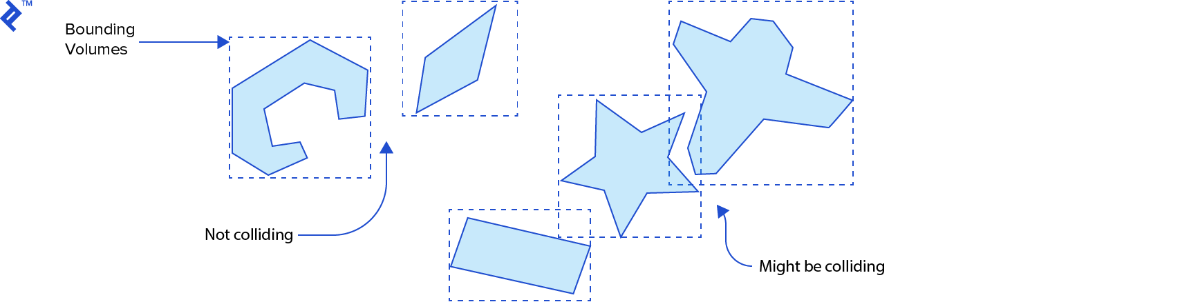
In the broad phase of collision physics for video games, we need to determine which pairs of rigid bodies might be colliding. These bodies can have intricate shapes like polygons and polyhedrons. To expedite this process, we can enclose each object within a simpler shape. If these bounding volumes don’t intersect, we can rule out any intersection between the actual shapes. If they do intersect, then the actual shapes might be intersecting.

Common types of bounding volumes include oriented bounding boxes (OBB), circles in 2D, and spheres in 3D. Let’s examine one of the simplest bounding volumes: axis-aligned bounding boxes (AABB).

AABBs are favored by physics programmers for their simplicity and advantageous trade-offs. A 2-dimensional AABB can be represented by a struct like this in the C language:

1
2
3
4
5
6
7
8
9

typedef struct {
    float x;
    float y;
} Vector2;

typedef struct {
    Vector2 min;
    Vector2 max;
} AABB;

The min field represents the coordinates of the box’s bottom left corner, while the max field represents the top right corner.

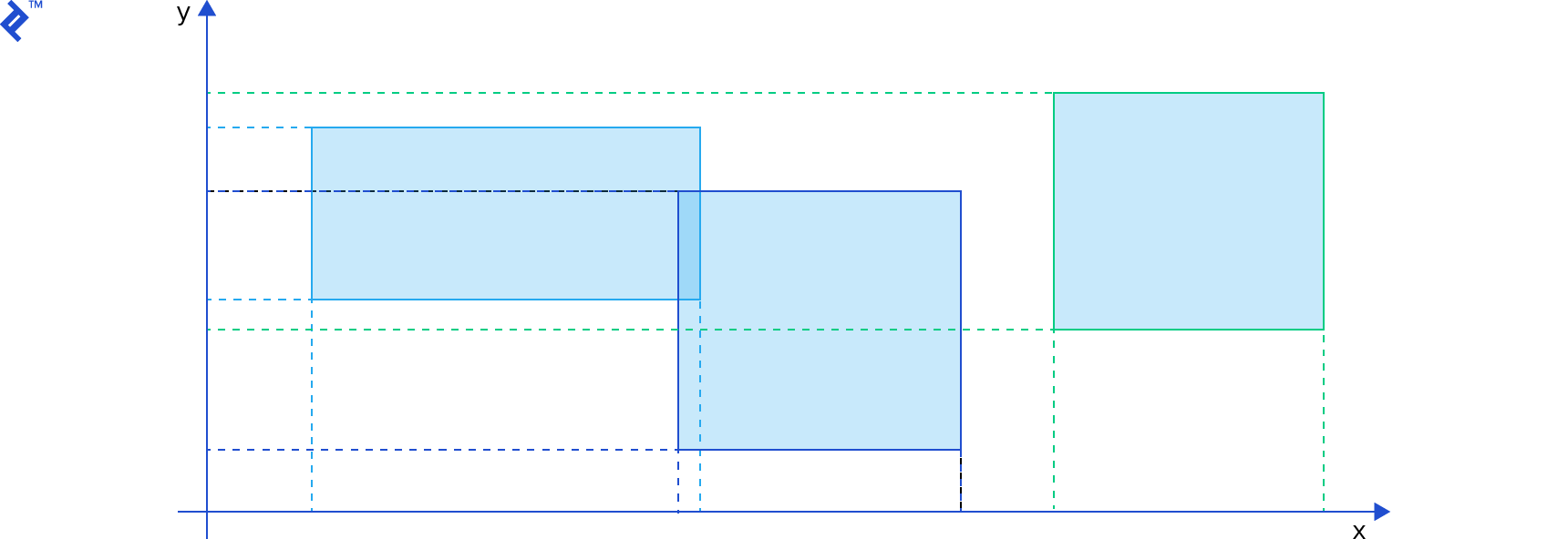
To determine if two AABBs intersect, we simply need to check if their projections overlap on all coordinate axes:

 1
 2
 3
 4
 5
 6
 7
 8
 9
10
11
12
13
14
15

BOOL TestAABBOverlap(AABB* a, AABB* b)
{
    float d1x = b->min.x - a->max.x;
    float d1y = b->min.y - a->max.y;
    float d2x = a->min.x - b->max.x;
    float d2y = a->min.y - b->max.y;

    if (d1x > 0.0f || d1y > 0.0f)
        return FALSE;

    if (d2x > 0.0f || d2y > 0.0f)
        return FALSE;

    return TRUE;
}

This code mirrors the logic of the b2TestOverlap function from the Box2D engine (version 2.3.0). It computes the difference between the min and max values of both AABBs, across both axes, and in both orders. If any of these differences are positive, the AABBs don’t intersect.

Despite the efficiency of an AABB overlap test, if we still perform pairwise tests for every possible pair, we encounter the unfavorable O(_n_2) time complexity. To minimize the number of AABB overlap tests, we can employ a space partitioning, operating on similar principles as the database indices used to accelerate queries. (Geographical databases, such as PostGIS, utilize comparable data structures and algorithms for spatial indexing.) However, the AABBs in our case are constantly moving, often requiring index recreation after each simulation step.

Numerous space partitioning algorithms and data structures are suitable for this purpose, including uniform grids, quadtrees in 2D, octrees in 3D, and spatial hashing. Let’s delve into two prevalent spatial partitioning algorithms: sort and sweep, and bounding volume hierarchies (BVH).

The Sort and Sweep Algorithm

The sort and sweep method (also known as sweep and prune) is a preferred choice among physics programmers for rigid body simulations. The Bullet Physics engine, for instance, implements this method in its btAxisSweep3 class.

Projecting an AABB onto a single coordinate axis essentially yields an interval [b, e] (representing beginning and end). With numerous rigid bodies in our simulation, we have many AABBs and consequently, many intervals. Our goal is to identify the intersecting intervals.

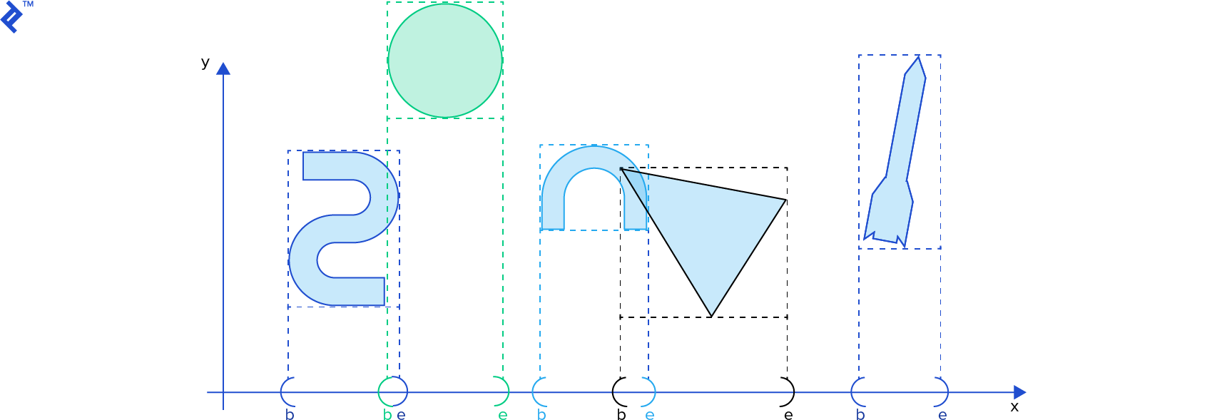
In the sort and sweep algorithm, we compile all b and e values into a single list, sorting it in ascending order based on their scalar values. We then sweep or traverse this list. When a b value is encountered, its corresponding interval is added to a separate active intervals list. Conversely, when an e value is encountered, its corresponding interval is removed from the active intervals list. At any given moment, all intervals in the active intervals list are intersecting. (Refer to David Baraff’s Ph. D Thesis](http://www.cs.cmu.edu/~baraff/papers/thesis-part1.ps.Z), p. 52 for a detailed explanation. Using this online tool to view the postscript file is recommended.) This interval list can be reused in subsequent simulation steps, allowing efficient resorting using [insertion sort], which excels at sorting nearly-sorted lists.

In two and three dimensions, applying the sort and sweep along a single coordinate axis reduces the number of direct AABB intersection tests. However, the performance gain might vary depending on the chosen axis. Consequently, more sophisticated variations of the sort and sweep algorithm are employed. In his book Real-Time Collision Detection (page 336), Christer Ericson presents an efficient variation. This variation stores all AABBs in a single array. For each sort and sweep iteration, one coordinate axis is selected, and the array is sorted based on the min value of the AABBs along the chosen axis using quicksort. The array is then traversed, and AABB overlap tests are performed. To determine the next sorting axis, the variance of the AABB centers is calculated, and the axis with the largest variance is chosen for the next step.

Dynamic Bounding Volume Trees

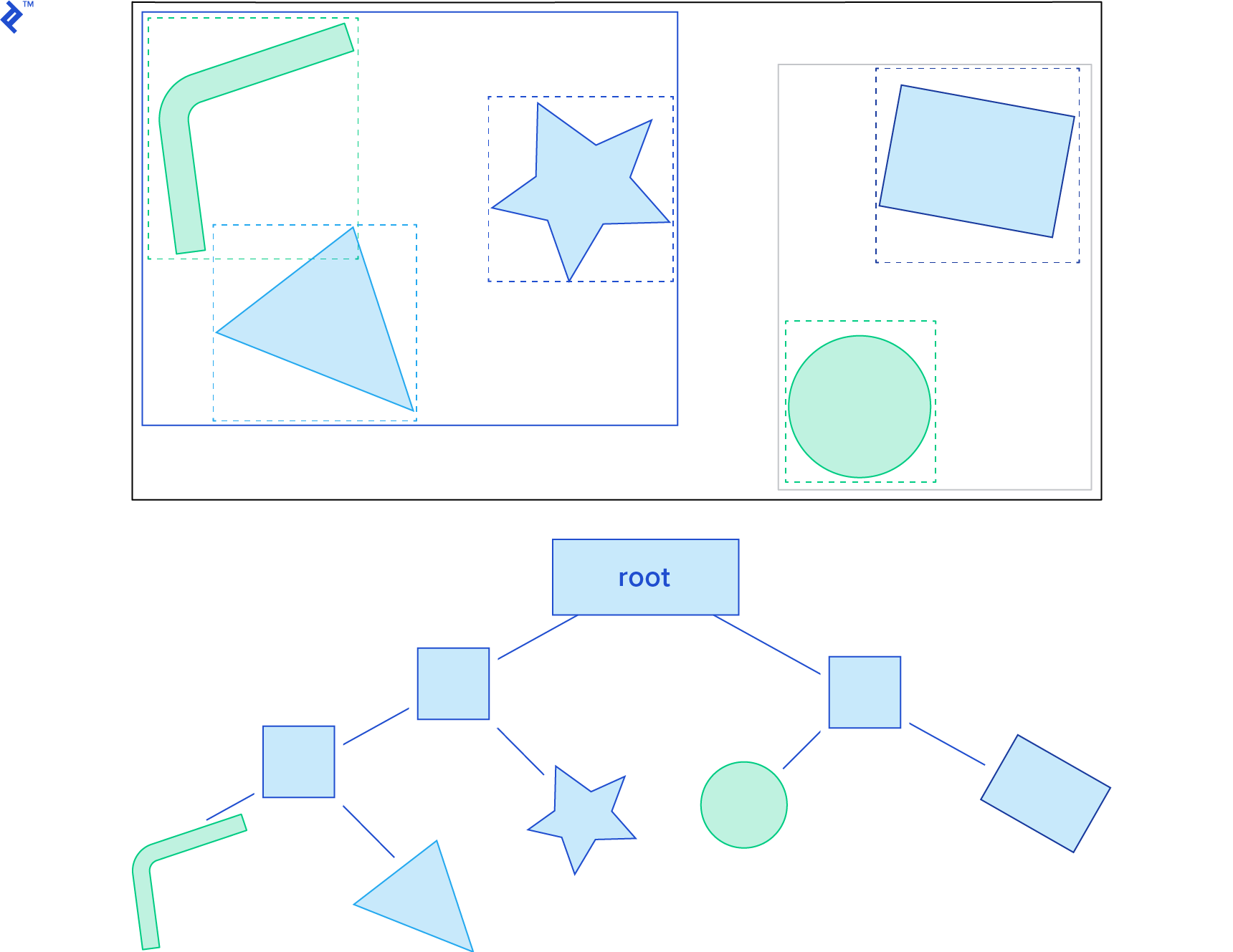
Another effective spatial partitioning method is the dynamic bounding volume tree, or Dbvt. This is a type of bounding volume hierarchy.

The Dbvt is a binary tree where each node possesses an AABB encompassing the AABBs of its children. The AABBs of the rigid bodies themselves reside in the leaf nodes. Typically, a Dbvt is “queried” by providing the AABB for which we want to detect intersections. This operation is efficient because we can disregard the children of nodes whose AABBs don’t intersect with the queried AABB. Therefore, an AABB collision query begins at the root and recursively traverses the tree, examining only the AABB nodes that intersect with the queried AABB. The tree can be balanced through tree rotations, similar to an AVL tree.

Box2D features a sophisticated Dbvt implementation in its b2DynamicTree class. The b2BroadPhase class handles the broad phase, utilizing a b2DynamicTree instance to execute AABB queries.

Narrow Phase

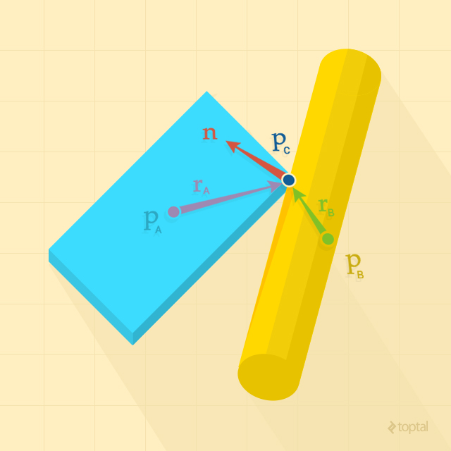
Following the broad phase, we obtain a set of rigid body pairs that are potentially colliding. In the narrow phase, for each pair, we need to determine if they are actually colliding based on their shape, position, and orientation. This involves checking for intersection or if their distance falls below a predefined tolerance. Additionally, we need to identify the contact points between colliding bodies, which are essential for subsequent collision resolution.

Convex and Concave Shapes

Determining if two arbitrary shapes intersect or calculating the distance between them is generally not straightforward in video game physics. However, one crucial factor influencing the difficulty is the shape’s convexity. Shapes can be either convex or concave, with concave shapes presenting greater challenges, necessitating specific strategies.

In a convex shape, any line segment connecting two points within the shape lies entirely within the shape. However, this doesn’t hold true for all possible line segments in a concave shape. If at least one line segment connecting points within the shape falls outside the shape, it’s classified as concave.

Computationally, it’s advantageous to have all shapes in a simulation represented as convex. This is because numerous powerful distance and intersection test algorithms are designed for convex shapes. However, not all objects are inherently convex, and we typically address this using two approaches: convex hull and convex decomposition.

The convex hull of a shape represents the smallest convex shape that fully encloses it. For a concave polygon in two dimensions, imagine placing a nail at each vertex and stretching a rubber band around all the nails. To compute the convex hull of a polygon, polyhedron, or a set of points, the quickhull algorithm is a suitable choice, boasting an average time complexity of O(n log n).

Representing a concave object with its convex hull results in the loss of its concave characteristics. This can lead to undesirable behavior like “ghost” collisions, as the object’s graphical representation remains concave. For instance, a car, typically concave, represented by its convex hull might exhibit a floating box if a box is placed on top of it.

Often, convex hulls suffice for representing concave objects, either because the unrealistic collisions are imperceptible or the concave properties are inconsequential to the simulation. However, in certain scenarios, we might require the concave object to behave as such physically. For example, using a convex hull to represent a bowl wouldn’t allow us to place anything inside it; objects would simply hover above. In such cases, we can utilize a convex decomposition of the concave shape.

Convex decomposition algorithms take a concave shape and generate a set of convex shapes whose union replicates the original concave shape. Representing some concave shapes might require a large number of convex shapes, potentially leading to significant computational overhead. However, an approximation often suffices, and algorithms like V-HACD can generate a small set of convex polyhedrons from a concave polyhedron.

In many collision physics scenarios, artists can manually perform convex decomposition, eliminating the performance cost of decomposition algorithms. Given the criticality of performance in real-time simulations, employing simplified physical representations for complex graphic objects is generally advisable. The following image illustrates a possible convex decomposition of a 2D car using nine convex shapes.

Testing for Intersections - The Separating Axis Theorem

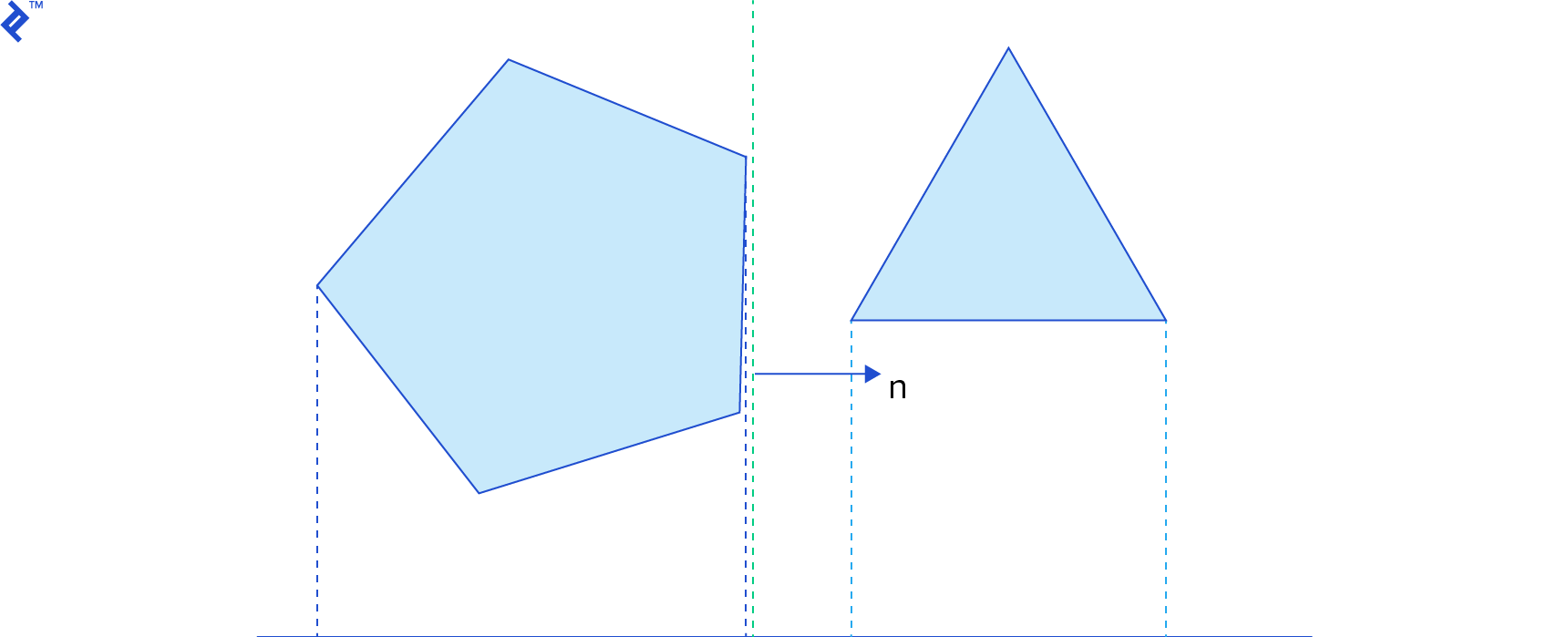
The separating axis theorem (SAT) posits that two convex shapes don’t intersect if and only if there exists at least one axis along which their orthogonal projections don’t overlap.

Visualizing a separating line in 2D or a plane in 3D that separates the two shapes is often more intuitive, representing the same principle. A vector orthogonal to the line in 2D, or the normal vector of the plane in 3D, serves as the “separating axis”.

Game physics engines handle various shape classes, including circles (spheres in 3D), edges (line segments), and convex polygons (polyhedrons in 3D), employing specific collision detection algorithms for each shape pair. The simplest is likely the circle-circle algorithm:

 1
 2
 3
 4
 5
 6
 7
 8
 9
10
11
12
13
14

typedef struct {
    float centerX;
    float centerY;
    float radius;
} Circle;

bool CollideCircles(Circle *cA, Circle *cB) {
    float x = cA->centerX - cB->centerX;
    float y = cA->centerY - cB->centerY;
    float centerDistanceSq = x * x + y * y; // squared distance
    float radius = cA->radius + cB->radius;
    float radiusSq = radius * radius;
    return centerDistanceSq <= radiusSq;
}

While SAT applies to circles, checking if the distance between their centers is less than the sum of their radii is much simpler. Consequently, SAT is employed in collision detection algorithms for specific shape class pairs, such as convex polygon against convex polygon (or polyhedrons in 3D).

For any shape pair, infinitely many axes could be tested for separation. Efficient SAT implementation hinges on determining the first test axis. When testing convex polygon intersection, we can utilize edge normals as potential separating axes. The normal vector n of an edge is perpendicular to the edge vector, pointing outward from the polygon. For each edge of each polygon, we simply need to check if all vertices of the other polygon lie in front of the edge.

If any test passes – that is, if for any edge, all vertices of the other polygon are in front of it – then the polygons don’t intersect. Linear algebra provides a straightforward formula for this test: given an edge on the first shape with vertices a and b and a vertex v on the other shape, if (v - a) · n is positive, the vertex lies in front of the edge.

For polyhedrons, we can utilize face normals and the cross product of all edge combinations from each shape. While this seems like numerous tests, we can optimize by caching the last separating axis used and attempting to reuse it in subsequent simulation steps. If the cached separating axis no longer separates the shapes, we can search for a new axis starting from faces or edges adjacent to the previous ones. This approach leverages the observation that bodies often exhibit limited movement or rotation between steps.

Box2D utilizes SAT to determine convex polygon intersection in its polygon-polygon collision detection algorithm, implemented in b2CollidePolygon.cpp.

Computing Distance - The Gilbert-Johnson-Keerthi Algorithm

Often, we want to consider objects as colliding not only upon intersection but also when they are very close, requiring distance computation. The Gilbert-Johnson-Keerthi (GJK) algorithm calculates the distance between two convex shapes and identifies their closest points. It’s an elegant algorithm leveraging an implicit representation of convex shapes through support functions, Minkowski sums, and simplexes.

Support Functions

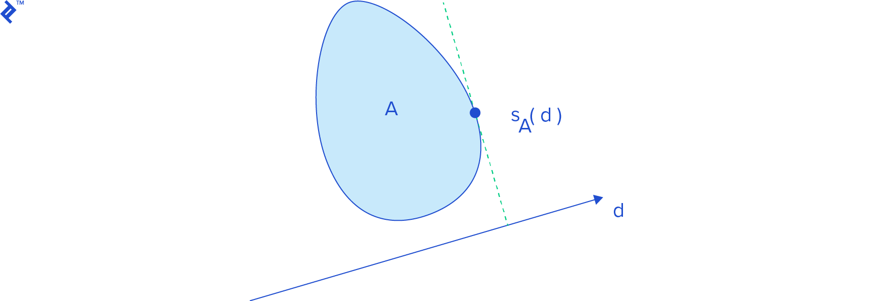
A support function s_A(d_) returns a point on shape A’s boundary with the highest projection onto vector d, mathematically represented by the highest dot product with d. This point is called a support point, and the operation is known as support mapping. Geometrically, it represents the farthest point on the shape in d’s direction.

Finding a polygon’s support point is relatively straightforward. For a support point for vector d, we iterate through its vertices and identify the one with the highest dot product with d:

 1
 2
 3
 4
 5
 6
 7
 8
 9
10
11
12
13
14
15
16

Vector2 GetSupport(Vector2 *vertices, int count, Vector2 d) {
    float highest = -FLT_MAX;
    Vector2 support = (Vector2){0, 0};

    for (int i = 0; i < count; ++i) {
        Vector2 v = vertices[i];
        float dot = v.x * d.x + v.y * d.y;

        if (dot > highest) {
            highest = dot;
            support = v;
        }
    }

    return support;
}

The power of support functions lies in simplifying operations with shapes like cones, cylinders, and ellipses. Directly computing the distance between such shapes is complex, and without GJK, we’d typically resort to discretizing them into polygons or polyhedrons, which can introduce other issues. Polyhedron surfaces lack the smoothness of surfaces like spheres unless highly detailed, potentially impacting collision detection performance. Additionally, undesirable side effects might arise; for instance, a “polyhedral” sphere might not roll smoothly.

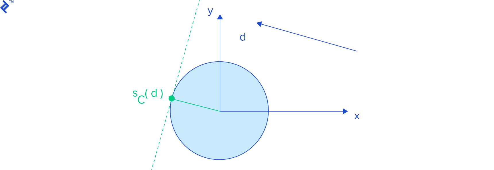
To obtain a support point for a sphere centered at the origin, we normalize d (compute d / ||d||, a unit vector in d’s direction) and multiply it by the sphere’s radius.

Refer to Gino van den Bergen’s paper for more examples of support functions for various shapes, including cylinders and cones.

In our simulation space, objects are displaced and rotated from the origin. We employ an affine transformation T(x) = Rx + c for this purpose, where c represents the displacement vector and R is the rotation matrix. This transformation first rotates the object about the origin and then translates it. The support function for a transformed shape A is:

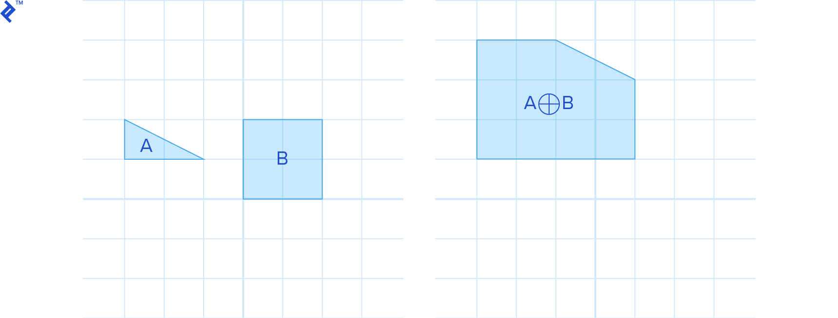
Minkowski Sums

The Minkowski sum of two shapes, A and B, is defined as:

This involves computing the sum for all points within A and B. The result resembles inflating A with B.

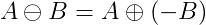
Similarly, the Minkowski difference is defined as:

which can also be expressed as the Minkowski sum of A and -B:

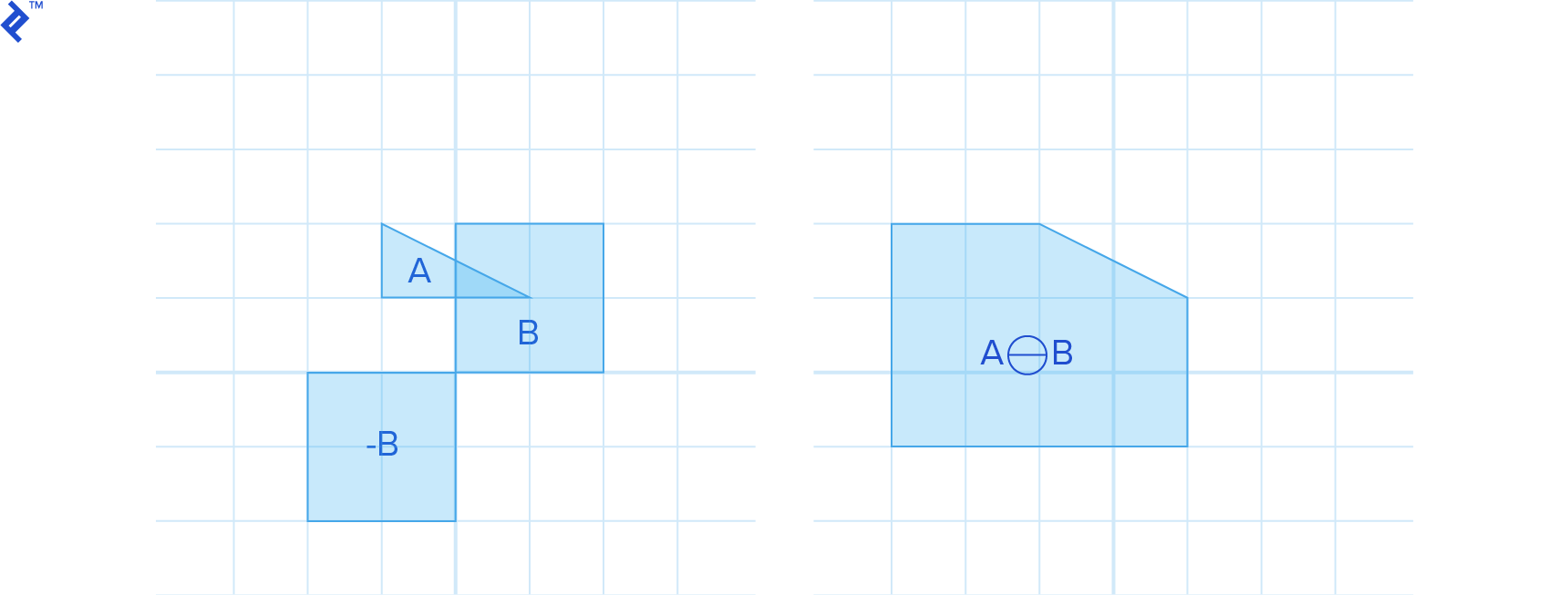
For convex shapes A and B, their Minkowski sum A⊕B is also convex.

A key property of the Minkowski difference is that if it contains the origin, the shapes intersect. This is because intersecting shapes share at least one point with the same spatial location, resulting in a zero vector difference, which corresponds to the origin.

Another useful characteristic is that if the Minkowski difference doesn’t contain the origin, the minimum distance between the origin and the Minkowski difference represents the distance between the shapes.

The distance between two shapes is defined as:

In other words, it’s the length of the shortest vector connecting A and B. This vector lies within A⊖B and is the shortest, hence closest to the origin.

Explicitly constructing the Minkowski sum of two shapes is generally not straightforward. Fortunately, we can again leverage support mapping:

Simplexes

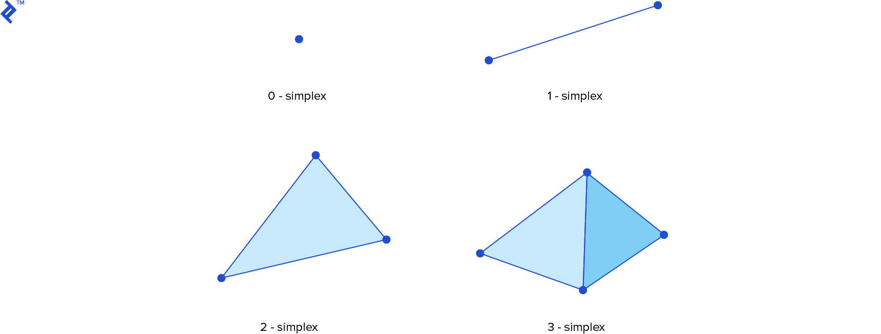
The GJK algorithm iteratively searches for the point on the Minkowski difference closest to the origin. It achieves this by constructing a series of simplexes that progressively approach the origin with each iteration. A simplex – more specifically, a k-simplex for an integer k – is the convex hull of k + 1 affinely independent points in a k-dimensional space. This implies that two points must be distinct, three points must not be collinear, and four points must not be coplanar. Consequently, a 0-simplex is a point, a 1-simplex is a line segment, a 2-simplex is a triangle, and a 3-simplex is a tetrahedron. Removing a point from a simplex reduces its dimensionality by one, while adding a point increases it by one.

GJK in Action

Let’s combine these concepts to understand GJK’s workings. To determine the distance between shapes A and B, we begin by considering their Minkowski difference, A⊖B. Our goal is to find the point on this resulting shape closest to the origin, as its distance represents the distance between the original shapes. We choose an arbitrary point v within A⊖B as our initial distance approximation and define an empty point set W to store the points of the current test simplex.

We then enter a loop. First, we obtain the support point w = sA⊖B(-v), the point on A⊖B whose projection onto v is closest to the origin.

If ||w|| is very close to ||v|| and the angle between them hasn’t changed significantly (based on predefined tolerances), the algorithm has converged. We can then return ||v|| as the distance.

Otherwise, we add w to W. If the convex hull of W (the simplex) contains the origin, the shapes intersect, and we’re done. If not, we find the point within the simplex closest to the origin and update v to this new closest approximation. We then remove any points from W that don’t contribute to the closest point computation (e.g., if the closest point to the origin lies on an edge of a triangle, we remove the vertex not belonging to that edge). These steps repeat until convergence.

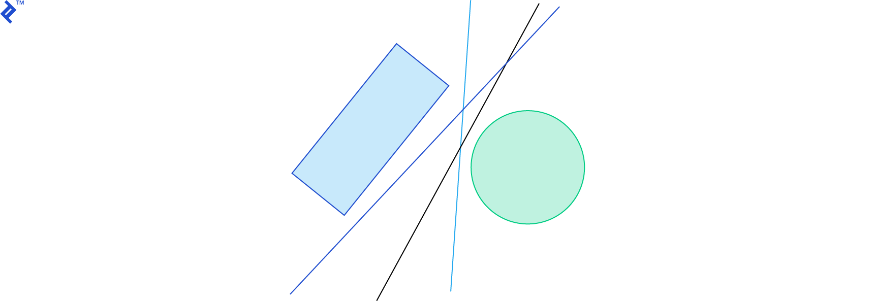
The following image illustrates four iterations of the GJK algorithm. The blue object represents the Minkowski difference A⊖B, and the green vector is v. Observe how v progressively approaches the point closest to the origin.

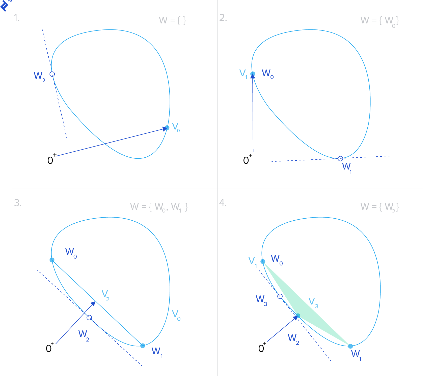
For an in-depth explanation of the GJK algorithm, refer to the paper A Fast and Robust GJK Implementation for Collision Detection of Convex Objects by Gino van den Bergen. The blog for the dyn4j physics engine also provides a great post on GJK.

Box2D implements the GJK algorithm in b2Distance.cpp within the b2Distance function. However, it utilizes GJK only during time of impact computation for continuous collision detection, a topic we’ll revisit later.

The Chimpunk physics engine relies on GJK for all collision detection. Its implementation is found in cpCollision.c within the GJK function. Upon detecting an intersection using GJK, it requires the contact points and penetration depth, which it obtains using the Expanding Polytope Algorithm, discussed next.

Determining Penetration Depth - The Expanding Polytope Algorithm

As previously mentioned, if shapes A and B intersect, GJK produces a simplex W containing the origin within the Minkowski difference A⊖B. This indicates intersection, but many collision detection systems benefit from knowing the intersection extent and the contact points for realistic collision handling. The Expanding Polytope Algorithm (EPA) provides this information, building upon GJK’s output: a simplex containing the origin.

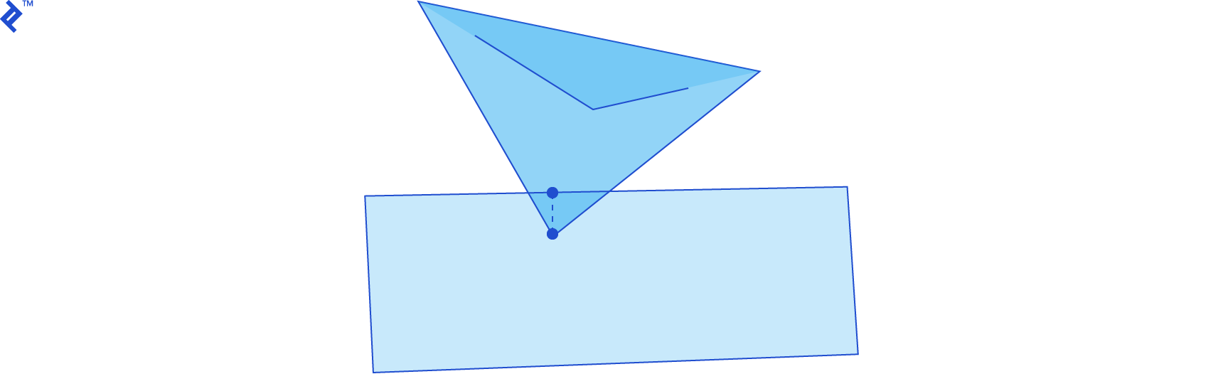
The penetration depth represents the length of the minimum translation vector (MTV), the smallest vector along which we can translate one intersecting shape to separate it from the other.

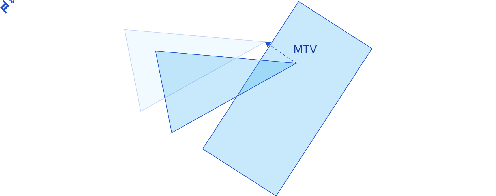
When two shapes intersect, their Minkowski difference contains the origin. The point on the Minkowski difference’s boundary closest to the origin represents the MTV. The EPA algorithm identifies this point by expanding GJK’s simplex into a polygon, iteratively subdividing its edges with new vertices.

First, we locate the simplex edge closest to the origin and compute the support point in the Minkowski difference along a direction normal to this edge (perpendicular and outward-pointing). We then split this edge by incorporating the support point. These steps repeat until the vector’s length and direction stabilize. Upon convergence, we obtain the MTV and penetration depth.

Combining GJK and EPA provides a comprehensive collision description, whether the objects intersect or are sufficiently close to be considered colliding.

The EPA algorithm is described in the paper Proximity Queries and Penetration Depth Computation on 3D Game Objects, also authored by Gino van den Bergen. The dyn4j blog offers a post about EPA on the topic.

Continuous Collision Detection

The techniques discussed so far perform collision detection on a static simulation snapshot, known as discrete collision detection. This approach disregards events between consecutive steps, potentially missing collisions, especially for fast-moving objects. This issue is referred to as tunneling.

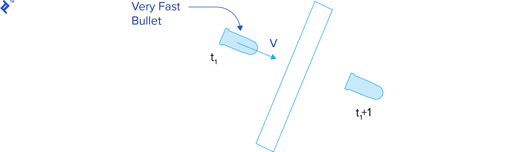
Continuous collision detection techniques aim to determine when a collision occurred between the previous and current simulation steps. They compute the time of impact, allowing us to rewind and process the collision at the precise moment.

The time of impact (or time of contact) t__c represents the instant when the distance between two bodies becomes zero. Given a function describing the distance between two bodies over time, we seek the smallest root of this function. Therefore, time of impact computation is essentially a root-finding problem problem.

For this computation, we consider the body’s state (position and orientation) at the previous step, time t__i-1, and the current step, time t__i. We assume linear motion between these steps for simplification.

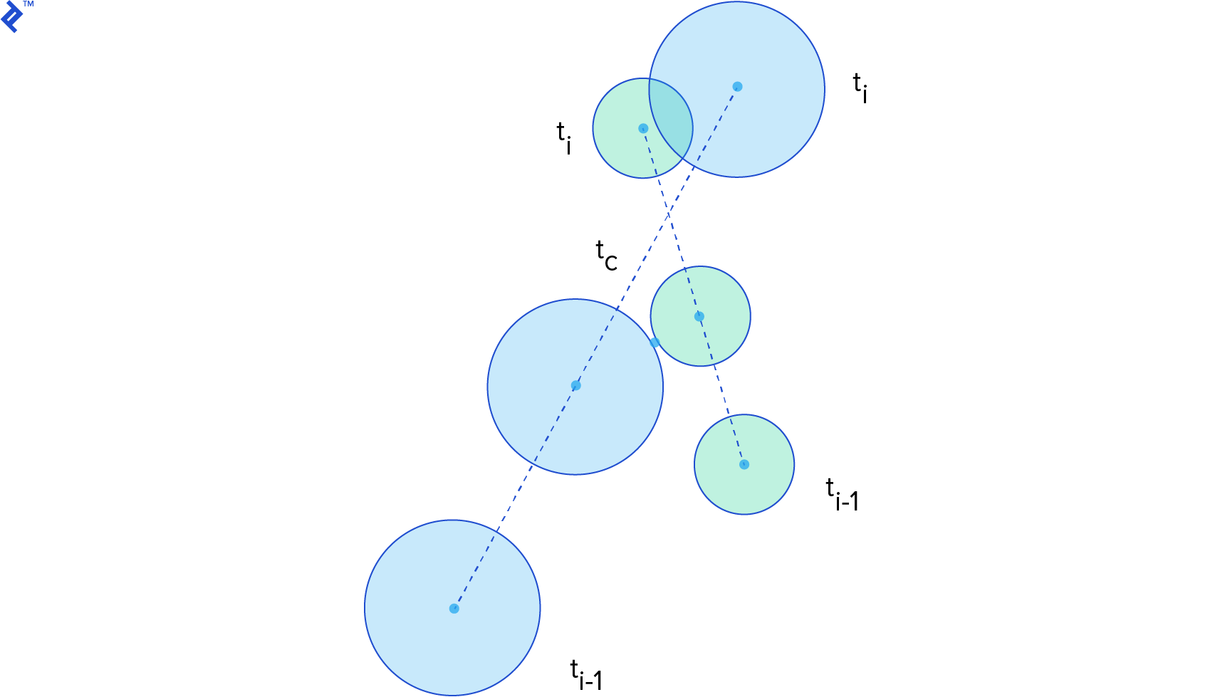
Let’s further simplify by considering circular shapes. For circles _C_1 and _C_2 with radii _r_1 and _r_2, where their centers of mass _x_1 and _x_2 coincide with their centroids, the distance function is:

Assuming linear motion, _C_1’s position from t__i-1 to t__i is:

This represents a linear interpolation between _x_1(t__i-1) and _x_1(t__i). The same applies to _x_2. Within this interval, the distance function becomes:

Setting this expression to zero yields a quadratic equation in t. We can directly solve for the roots using the quadratic formula. If the circles don’t intersect, the quadratic formula won’t have a solution. Otherwise, it might yield one or two roots. A single root represents the time of impact. With two roots, the smaller one represents the time of impact, while the larger one indicates the time of separation. Note that the time of impact is a value between 0 and 1, representing a fraction of the time step rather than seconds. It’s used to interpolate the bodies’ states to the exact collision point.

Continuous Collision Detection for Non-Circles

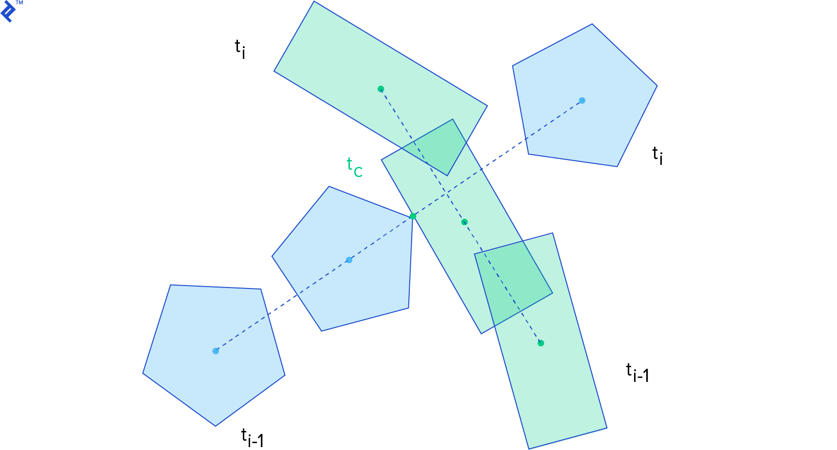
Formulating distance functions for other shapes is challenging because their distance depends on orientation. Consequently, we often rely on iterative algorithms that progressively move the objects closer until they are sufficiently close to be considered colliding.

The conservative advancement algorithm iteratively moves and rotates the bodies forward. In each iteration, it calculates an upper bound for displacement. The original algorithm, presented in Brian Mirtich’s PhD Thesis (section 2.3.2), accounts for ballistic motion. This paper by Erwin Coumans (creator of the Bullet Physics Engine) presents a simpler version using constant linear and angular velocities.

This algorithm determines the closest points between shapes A and B, constructs a vector connecting them, and projects the velocity onto this vector to determine an upper bound for motion. This ensures that no point on either body moves beyond this projection. The bodies are then advanced by this amount, and the process repeats until the distance falls below a small threshold.

Convergence might require many iterations, especially when one body has high angular velocity.

Resolving Collisions

Upon collision detection, we need to realistically modify the colliding objects’ motions, such as making them bounce off each other. The next and final installment in this series will explore common collision resolution methods employed in video games.

References

For a deeper dive into collision physics, including algorithms and techniques, Real-Time Collision Detection by Christer Ericson is an invaluable resource.

Given the reliance of collision detection on geometry, Toptal’s article, Computational Geometry in Python: From Theory to Application, serves as an excellent introduction.