If you’re like most Google Ads users, you’re probably familiar with the platform’s user interface (UI) and its abundance of reports. However, even seasoned professionals may find it challenging to extract meaningful insights from the sheer volume of data without the aid of clear visualizations. At nexus-security, we excel in designing custom dashboards that simplify the process of communicating goals to clients and teams. By automating this process whenever feasible, we can dedicate more time to optimizing your account’s performance.

This guide will walk you through the creation of visually appealing and functional Google Ads reporting dashboards that you can personalize with your own branding. While we encourage you to follow the steps outlined below, a pre-built Google Ads report template is available at the end for those seeking a ready-made solution.

Get a free, instant audit of your Google Ads account with our Google Ads Performance Grader today!

Extracting Your Google Ads Data

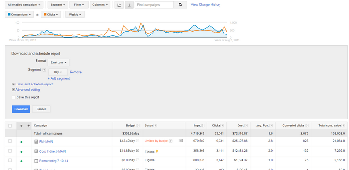
Start by defining your desired date range. If you’re creating a new report from scratch, feel free to go as far back as you need. In this instance, we’ll be analyzing data from 2014 to the present day. Ensure that your report includes only the following columns: Impressions, Clicks, Cost, Average Position, Converted Clicks, and Total Conversion Value (you have the option to use Conversions instead of Converted Clicks if required). Proceed to click the “Download” button and segment the data by “Day.” Add two more segmentations, one by “Week” and another by “Month.” Once you’ve configured these settings, download the report and open it.

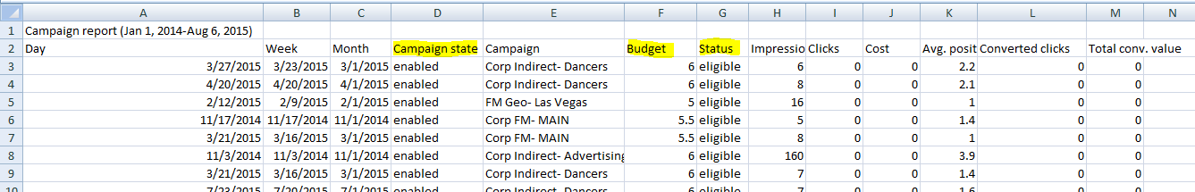
Your report should resemble the example provided above. Our next step involves removing a few unnecessary columns. To do so, click on the letter heading of the column you want to delete. For instance, to delete the “Campaign state” column, click on the letter “D.” Instead of using the “delete” key to remove the column, we’ll use the keyboard shortcut “Ctrl & -” to delete the entire row. Repeat this process for the other highlighted columns. After deleting these columns, you should be left with the following: Day, Week, Month, Campaign, Impressions, Clicks, Cost, Avg Position, Converted Clicks, and Total Conv. Value.

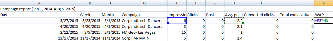
Let’s add a formula to calculate a more accurate representation of average position, specifically the Weighted Average Position (WAP). Create a new column titled “WAP” and in the first cell, enter the following formula: =Impressions * Avg Pos (In this example, it would be =E3*H3). Proceed to drag this formula down the entire data column (or double-click the small black box at the bottom right corner of the selected cell for an instant drop-down).

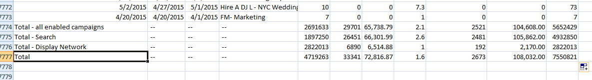
Delete the first row containing the date range using “Ctrl –”. Then, go to the bottom of the sheet and delete the four total rows (click on the number to the left of each row to select the entire row). Select cell A1, then navigate to the “Insert” option in the toolbar.

Creating the Pivot Table

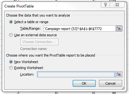
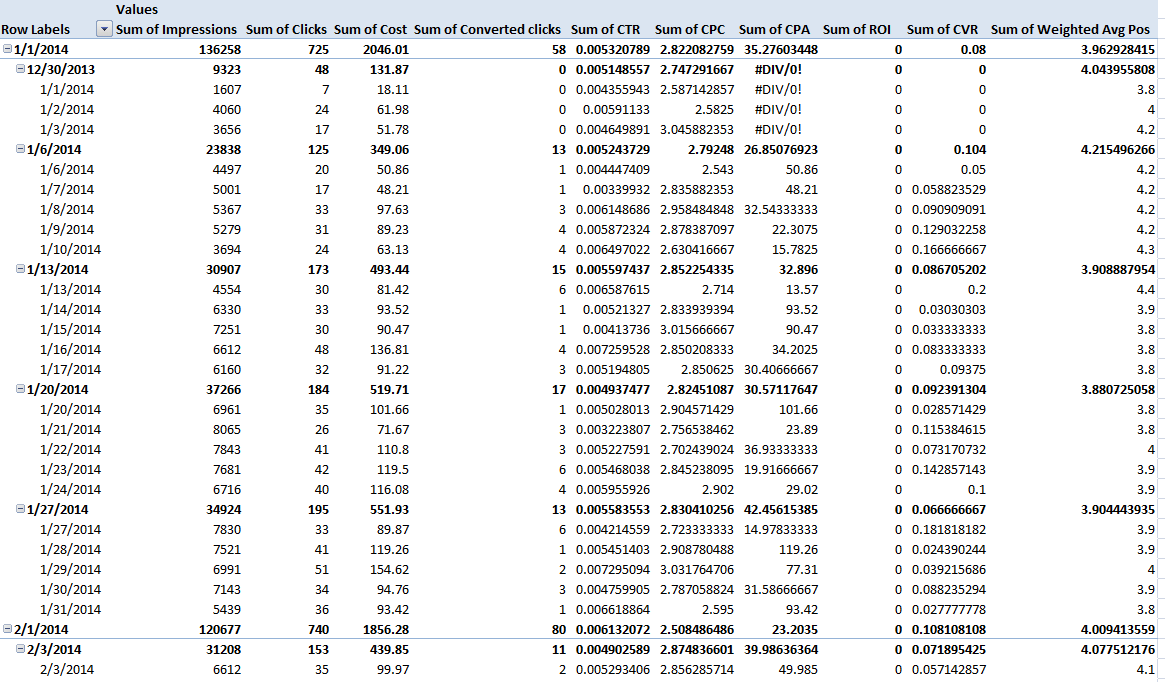
Since we’ll be using the default settings for the pivot table, simply click “OK”. You should now see an empty pivot table. Take this opportunity to grab your stress ball and give it a few squeezes — you’re about to realize that pivot tables are nothing to fear!

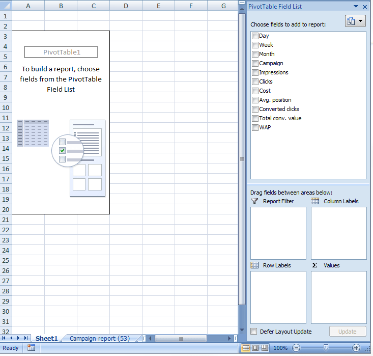
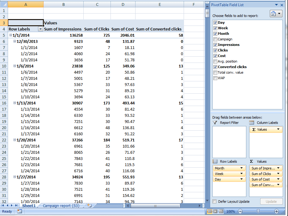
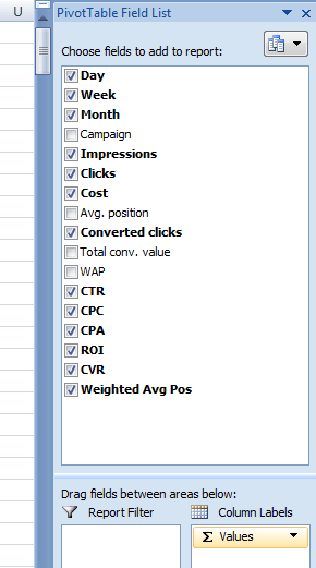
We’ve now added the initial set of metrics to our pivot table. These metrics are the ones that simply need to be summed up. For metrics that require multiplication or division (e.g., CTR = Clicks / Impressions), we need to perform an additional step.

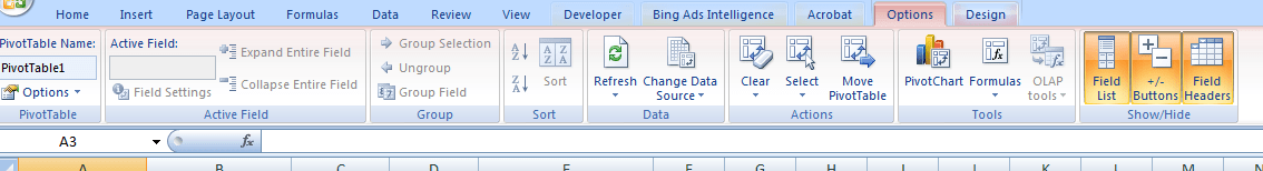
Go to the “Formulas” tab and select “Calculated Field”:

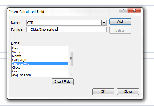
Create the following calculated fields with the corresponding formulas:

• CTR = Clicks / Impressions
• CPC = Cost / Clicks
• CPA = Cost / Converted Clicks
• ROI = Total Conversion Value / Cost
• CVR = Converted Clicks / Clicks
• Weighted Avg Pos = WAP / Impressions

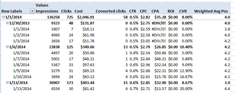
We’re making great progress! However, our table still lacks visual appeal. Presenting this to a client or your board of directors in its current state might not be the best idea. Let’s polish things up a bit.

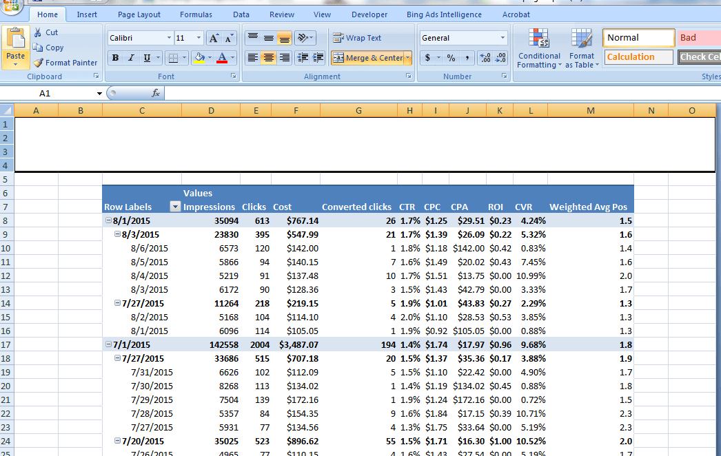
Currently, our columns are named “Sum Of XXXX”. Let’s rename them to their appropriate names and units. In the values area, click the drop-down arrow next to the first metric, “Impressions,” and select “Value Field Settings”:

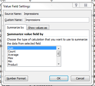
Change the name to “Impressions” (make sure to add a space after the word). Next, go to the “Number Format” tab:

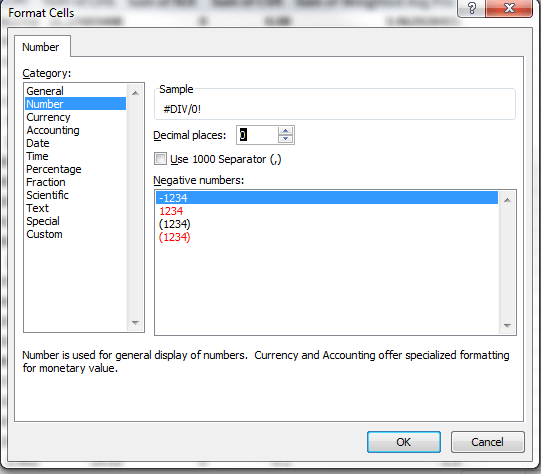
For Impressions, select “Number” with 0 decimal places. Repeat the same process for the remaining metrics using the following format settings:

• Clicks: Number, 0
• Cost: Currency, 2
• Converted Clicks: Number, 0
• CTR: Percentage, 1
• CPC: Currency, 2
• CPA: Currency, 2
• ROI: Currency, 2
• CVR: Percentage, 2
• Weighted Avg Pos: Number, 1

That’s looking much better! Now let’s arrange our data so that the most recent data appears at the top.

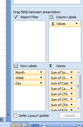
In the right panel, click on “Month” and choose “Sort Newest to Oldest”. Repeat this step for both “Week” and “Day”.

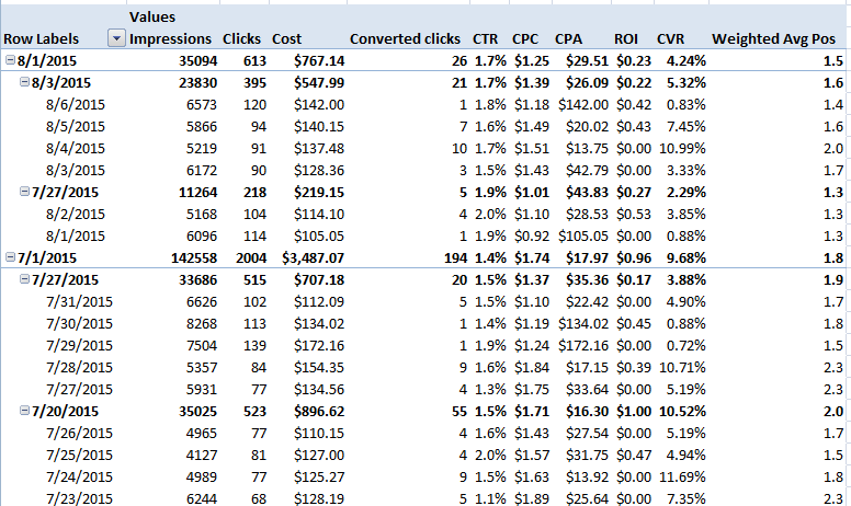
At this point, we can begin to identify trends within our data.

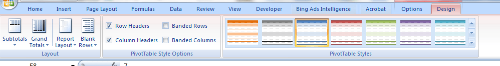
Let’s add some color to enhance the visual appeal. Go to the “Design” tab and select a color scheme that you find aesthetically pleasing. Next, add a few columns to the left of the pivot table and a few rows above it. Highlight a column above the pivot table, hold down “Ctrl Shift” and press the right arrow key to select all columns to the right. Right-click on any of the highlighted column headers and select “Hide.”

Highlight the top few rows above the pivot table. Then, in the “Home” tab, click on “Merge & Center.” We recommend matching the color of this merged header cell to the color scheme of the pivot table. Finally, type in the name of your client.

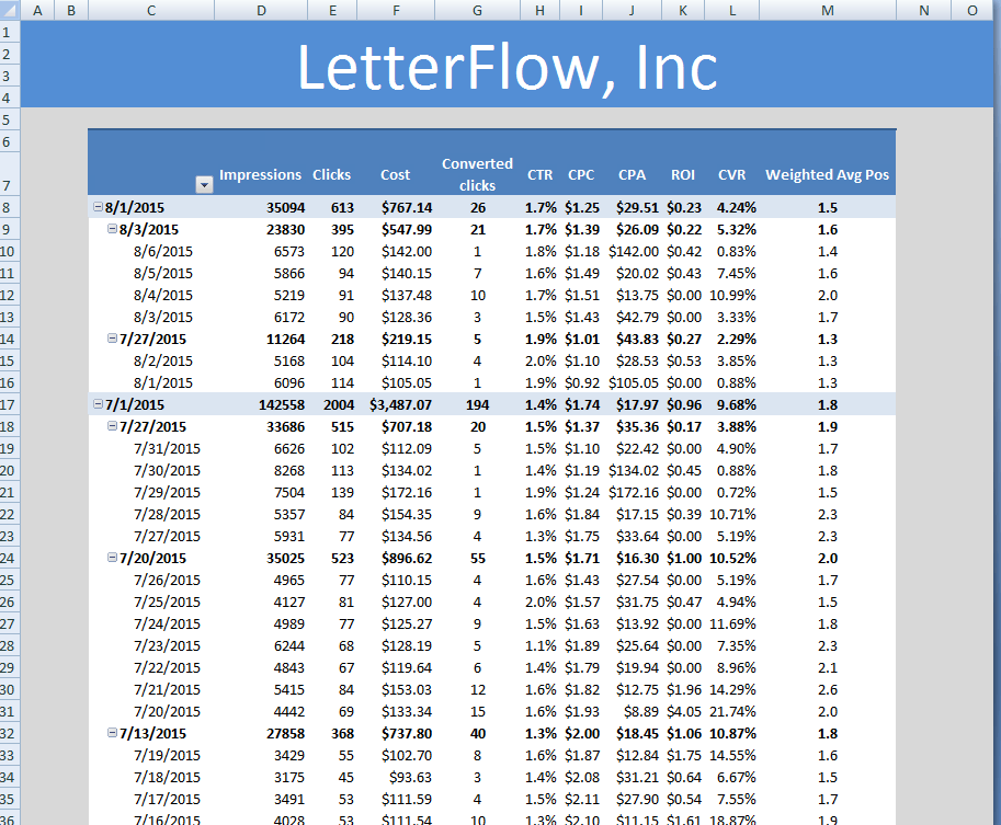
And there you have it! In just 15 minutes, we’ve created a professional-looking Google Ads report that’s ready to be shared with your clients. If you’d like to save time and utilize a pre-built template, click here to download a free PPC report template.