A network or graph is a structure used to represent data using nodes and the connections, called edges or links, between them. Both nodes and edges can possess various attributes, such as numerical values, categories, or even more intricate information.

Today, a vast quantity of data exists in the form of networks or graphs. This includes things like the World Wide Web, where web pages are nodes connected by hyperlink edges, social networks, semantic networks, biological networks, and citation networks within scientific literature, among many others.

Among graph types, a tree stands out as a specialized structure naturally suited to representing many forms of data. The field of computer and data science places significant emphasis on the analysis of trees. This article delves into the examination of link structures within trees, specifically focusing on tree kernels. Tree kernels offer a way to compare tree graphs, quantifying their similarities and differences. This process is crucial for various modern applications, including classification and data analysis.

Unsupervised Classification of Structured Data

Classification holds a significant place within machine learning and data analysis. It generally falls into two categories: supervised and unsupervised. In supervised classification, the classes are predefined, and a model learns from training data where the correct classes are already assigned. In contrast, unsupervised classification aims to uncover hidden categories when none are known beforehand. It achieves this by grouping data based on a measure of similarity.

When combined with graph theory, unsupervised classification can be used to identify groups of similar tree networks. Tree data structures are valuable for modeling objects in various domains. For instance, in natural language processing (NLP), parse trees, represented as ordered, labeled trees, are used to model sentence structure. In automated reasoning, problems often involve searching a space represented as a tree, with nodes representing search states and edges representing inference steps. Additionally, semistructured data, such as HTML and XML documents, lend themselves well to being modeled as ordered, labeled trees.

These domains benefit from the application of unsupervised classification techniques. For example, in NLP, classification can automatically categorize sentences into questions, commands, and statements. Similarly, by applying classification to their HTML source code, groups of websites with similar structures can be identified. The key requirement in these scenarios is a way to quantify the “similarity” between any two trees.

The Curse of Dimensionality

Many classification algorithms necessitate transforming data into a vectorized form. This vector representation reflects the values of the data’s features within a feature space, enabling analysis using linear algebra. For structured or semi-structured data like trees, the dimensionality of these vectors (the number of features in the feature space) can become quite large to accommodate the structural information.

This high dimensionality can be a significant obstacle since many classification techniques struggle to scale effectively as the number of dimensions grows. In other words, their ability to classify accurately diminishes as the input dimensionality increases, a problem known as the curse of dimensionality.

To grasp the reason behind this performance decline, imagine a space X with d dimensions containing a set of uniformly distributed points. As the number of dimensions in X increases, maintaining the same density of points requires an exponential increase in their number. Put simply, the more dimensions the input has, the more likely it is that the data becomes sparse. Sparse datasets pose a challenge for building reliable classifiers because the correlations between data points become too weak for algorithms to detect effectively.

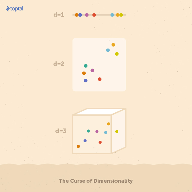
For example, each feature space depicted above contains eight data points. Identifying the group of five points on the left and the three on the right is straightforward in the one-dimensional space. However, as these points are spread across a higher number of features (i.e., dimensions), finding these groups becomes increasingly difficult. It’s important to note that feature spaces in real-world applications can easily have hundreds of dimensions.

Using a vectorized representation for structured data is suitable when domain knowledge allows for the selection of a manageable set of features. When this knowledge is lacking, techniques capable of directly handling structured data without relying on vector space operations are preferable.

Kernel Methods

Kernel methods offer a way to circumvent the need for converting data into vector form. The sole information they require is a measure of similarity, referred to as a kernel, between each pair of items in a dataset. The function used to determine this similarity is called the kernel function. Kernel methods seek linear relationships within the feature space, essentially performing a dot product between two data points in this space. While feature design can still play a role in crafting effective kernel functions, kernel methods bypass direct manipulation of the feature space. It can be demonstrated that the dot product can be substituted with a kernel function as long as that function is a symmetric, positive semidefinite function capable of taking the data in its raw, untransformed form.

The key benefit of using kernel functions is the ability to analyze a vast feature space with a computational complexity that depends not on the size of this space but on the complexity of the kernel function itself. Consequently, kernel methods effectively sidestep the curse of dimensionality.

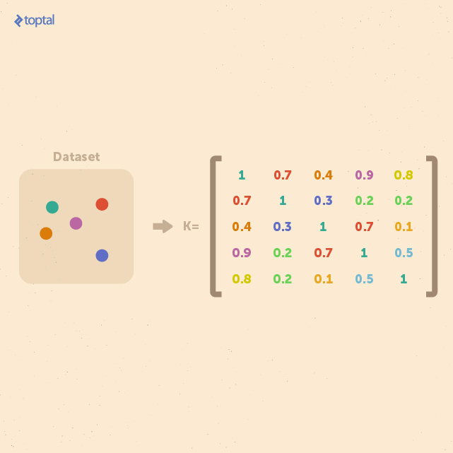
For a dataset containing n examples, a comprehensive representation of their similarities can be captured in a kernel matrix of size n × n. Crucially, this matrix remains independent of the size of individual examples, making it particularly advantageous for analyzing small datasets with high-dimensional features.

In essence, kernel methods take a different approach to data representation. Instead of mapping input points to a feature space, they represent data through pairwise comparisons within a kernel matrix K. All subsequent analysis can then be performed directly on this matrix.

The power of kernel methods extends to various data mining techniques, which can be “kernelized.” To classify instances of tree-structured data using methods like support vector machines, a valid (symmetric positive definite) kernel function k : T × T → R, known as a tree kernel, needs to be defined. Practically useful tree kernels should be computable in polynomial time with respect to the tree size and capable of detecting isomorphic graphs. These desirable tree kernels are called complete tree kernels.

Tree Kernels

Let’s delve into some practical tree kernels for gauging the similarity between trees. The core idea is to calculate the kernel value for each pair of trees in a dataset, ultimately constructing a kernel matrix that serves as the foundation for classifying sets of trees.

String Kernel

Before we proceed, a brief introduction to string kernels will prove useful, as it lays the groundwork for another kernel method based on transforming trees into strings.

Let’s define numy(s) as the count of occurrences of a substring y within a string s, where |s| represents the length of the string. The string kernel we’ll focus on is defined as follows:

Kstring(S1, S2) = Σs∈F nums(S1)nums(S2)ws

Here, F represents the set of substrings present in both strings, S1 and S2, and the parameter ws acts as a weight, allowing for the emphasis of specific substrings. This kernel assigns higher values to pairs of strings that share numerous common substrings.

Tree Kernel Based on Converting Trees into Strings

This string kernel can be leveraged to construct a tree kernel. The underlying concept involves systematically converting two trees into two strings, preserving their structural information, and then applying the string kernel described above.

The conversion of trees into strings follows this process:

Let T be one of the trees we aim to compare, and label(ns) represent the string label of node ns within T. Additionally, let tag(ns) denote the string representation of the subtree rooted at node ns in T. Consequently, if nroot is the root node of T, then tag(nroot) represents the entire tree T as a string.

Now, we can define string(T) = tag(nroot) as the complete string representation of T. To obtain this representation, we apply the following steps recursively in a bottom-up manner:

• If ns is a leaf node, tag(ns) is set to “[” + label(ns) + “]” (where + represents string concatenation).
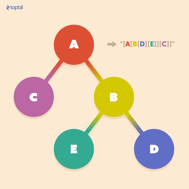
• If ns is not a leaf and has c children n1, n2, … , nc, we first obtain tag(n1), tag(n2), … , tag(nc). These are then lexicographically sorted to yield tag(n1*), tag(n2*), … , tag(nc* ). Finally, tag(ns) is set to “[” + label(ns) + tag(n1*) + tag(n2*) + … + tag(nc*) + “]”.

The following illustration showcases an example of this tree-to-string conversion. The outcome is a string enclosed in delimiters (e.g., “[” and “]”), with each nested pair of delimiters corresponding to a subtree rooted at a specific node:

By applying this conversion to two trees, T1 and T2, we obtain two strings, S1 and S2, respectively. The string kernel described earlier can then be applied to these strings.

Thus, the tree kernel between T1 and T2 via strings S1 and S2 is given by:

Ktree(T1, T2) = Kstring( string(T1), string(T2) ) = Kstring(S1, S2) = Σs∈F nums(S1)nums(S2)ws

In practice, the weight parameter often takes the form w|s|, assigning weight based on the substring length |s|. Common weighting schemes for w|s| include:

• constant weighting (w|s| = 1)
• k-spectrum weighting (w|s| = 1 if |s| = k, and w|s| = 0 otherwise)
• exponential weighting (w|s| = λ|s| where 0 ≤ λ ≤ 1 represents a decay rate)

Calculating the kernel involves determining all common substrings F and counting their occurrences in S1 and S2. This well-studied substring finding problem can be efficiently solved in O(|S1| + |S2|) time using algorithms like suffix trees or suffix arrays. Assuming a constant maximum number of symbols (e.g., bits, bytes, characters) required to represent a node’s label, the lengths of the converted strings are |S1| = O(|T1|) and |S2| = O(|T2|). Consequently, the kernel function’s computational complexity is linear, O(|T1| + |T2|).

Tree Kernel Based on Subpaths

The previous tree kernel employed a horizontal, breadth-first approach for converting trees into strings. While straightforward, this method doesn’t allow for direct operation on the trees’ original structures.

This section introduces a tree kernel that focuses on the vertical structures within trees, enabling direct operation on their original form.

We begin by defining a subpath as a segment of a path originating from the root and leading to a leaf. The subpath set encompasses all such subpaths within a tree:

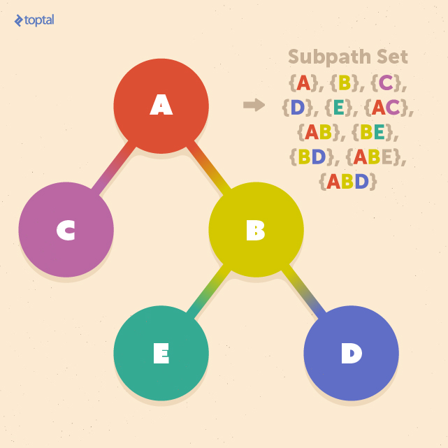
To define a tree kernel K(T1, T2) between two trees, T1 and T2, we can leverage the subpath set:

K(T1, T2) = Σp∈P nump(T1)nump(T2)w|p|

In this formula, nump(T) denotes the number of times subpath p appears in tree T, |p| represents the number of nodes in subpath p, and P encompasses all subpaths within both T1 and T2. Similar to the previous section, w|p| serves as the weight parameter.

Below is a basic implementation of this kernel using depth-first search. While this implementation has quadratic time complexity, more efficient algorithms employing suffix trees, suffix arrays, or extensions of the multikey quicksort algorithm can achieve linearithmic time ( O(|T1|log|T2|) ) on average:

 1
 2
 3
 4
 5
 6
 7
 8
 9
10
11
12
13
14
15
16
17
18
19
20
21
22
23
24
25
26
27
28
29
30
31
32
33
34
35
36
37

subpath_track = {}

def generate_subpaths(path, l):
  if l == len(path):
    if tuple(path) not in subpath_track:
      subpath_track[tuple(path)] = 1
    else:
      subpath_track[tuple(path)] += 1
  else:
    index = 0
    while l+index-1 < len(path):
      if tuple(path[index: l+index]) not in subpath_track:
        subpath_track[tuple(path[index: l+index])] = 1
      else:
        subpath_track[tuple(path[index: l+index])] += 1
      index += 1

    generate_subpaths(path, l+1)


def get_subpaths(graph, root, track, path):
  track[root] = True

  if graph.degree(root) == 1:
    generate_subpaths(path, 1)
  else:
    for node in graph.neighbors(root):
      if node not in track:
        get_subpaths(graph, node, track, path + [node, ])


def kernel_subpath(t1, t2, common_track):
  kernel_v = 0
  for p in subpath_track:
    kernel_v += common_track[t1][p]*common_track[t2][p]

  return kernel_v

In this implementation, the weight parameter w|p| is set to 1, giving equal weight to all subpaths. However, scenarios often arise where k-spectrum weighting or dynamically assigned weights are more appropriate.

Mining Websites

Before concluding, let’s explore a practical application of tree classification: categorizing websites. In data mining, knowing the “type” of website from which data originates can be highly beneficial. Due to the structural similarities in how web pages for similar services are designed, trees offer an effective way to categorize pages from different websites.

The key lies in the inherently nested structure of HTML documents, resembling that of trees. Each document has a single root element, with additional elements nested within. These nested elements are logically equivalent to child nodes in a tree representation:

Consider the following code snippet that converts an HTML document into a tree structure:

 1
 2
 3
 4
 5
 6
 7
 8
 9
10
11
12
13
14
15
16
17
18
19
20
21
22
23
24

def html_to_dom_tree(root):
  node_id = 1
  q = deque()
  graph = nx.Graph()

  q.appendleft({'element': root, "root_id": node_id})
  while len(q):
    node = q.pop()

    if node and node['element'].name == "body":
      graph.add_node(node_id, element=node['element'].name)
      node_id += 1

    root_id = node['root_id']
    labels[root_id] = node['element'].name

    for t in node['element'].contents:
      if t and t.name:
        graph.add_node(node_id, element=t.name)
        graph.add_edge(root_id, node_id)
        q.appendleft({"element": t, "root_id": node_id})
        node_id += 1

  return graph

Executing this code might result in a tree data structure similar to this:

The implementation above leverages two helpful Python libraries: NetworkX for working with graph structures, and Beautiful Soup for retrieving and processing web documents.

Calling the function html_to_dom_tree(soup.find("body")) produces a NetworkX graph object rooted at the <body> element of the webpage.

Now, suppose we want to identify groups within a set of 1,000 website homepages. We can convert each homepage into a tree using the method described above and then compare them using, for example, the subpath tree kernel from the previous section. These similarity measurements might reveal distinct clusters, allowing us to identify categories such as e-commerce websites, news sites, blogs, and educational sites based on their structural resemblance.

Conclusion

This article introduced methods for comparing tree-structured data, specifically focusing on how kernel methods can be applied to trees to quantify their similarity. Kernel methods excel in high-dimensional spaces, a common characteristic of tree structures. These techniques pave the way for further analysis of large tree datasets using well-established methods that operate on kernel matrices.

Tree structures are prevalent in various real-world domains, including XML and HTML documents, chemical compounds, natural language processing, and certain types of user behavior. As exemplified by constructing trees from HTML, these techniques provide us with powerful tools for conducting meaningful analyses in these areas.