Predicting the future is a key aspect of many disciplines, and it’s something we often call forecasting. By looking at past data and trends, we can make educated guesses about future outcomes, like potential disasters, shifts in behavior, or overall patterns in any subject. This information is incredibly valuable for making informed decisions, especially in a business setting where it can help estimate costs, project revenue, and create realistic budgets.

When it comes to the business world, there are two main types of forecasting: qualitative forecasting and quantitative forecasting.

• Qualitative forecasting: This approach is all about understanding the market. It relies heavily on expert opinions, market research, and takes human factors into account. Businesses typically use qualitative forecasting for short-term strategies.
• Quantitative forecasting: This method is all about the numbers. It ignores human intuition and relies solely on historical data to predict future outcomes for things like sales figures, price fluctuations, and other long-term financial factors.

For a deeper dive into the world of forecasting, Investopedia’s Financial Forecasting provides a great starting point.

Both qualitative and quantitative forecasting have proven to be incredibly valuable, leading to substantial improvements for many businesses.

If you want to explore how forecasting can impact market decisions, Prediction Markets: Fundamentals, Designs, and Applications by Stefan Luckner et al. is an excellent resource.

One area where quantitative forecasting really shines is in demand forecasting, also known as sales forecasting.

Predicting Demand and Forecasting Sales: A Closer Look

Imagine you’re a retailer managing numerous stores, each with a product restocking system based on human intuition and triggered by events like changing seasons or market trends. This system, while common, can lead to two major issues:

• Excess Inventory: You end up with a surplus of products that were meant to sell within a specific period but didn’t.
• Stock Shortages: You miss out on sales opportunities because you don’t have the desired products in stock.

A study by an IHL Group survey of 600 households and retailers revealed that retailers lose close to $1 trillion in sales each year due to stockouts.

According to the IHL Group, “Shoppers encounter out-of-stocks in as often as one in three shopping trips. At food, drug and mass retailers, they encounter out-of-stock items in one in five trips, at department store and specialty retailers it’s one in four, and at electronics stores one in three.”

As you can see, both excess inventory and stock shortages negatively impact revenue. Overstocking means tying up money in unsold goods, while understocking leads to missed sales opportunities. Both scenarios hurt a company’s cash flow. To mitigate this risk, two key elements are needed:

• More Data: Access to richer data sets can lead to better informed decisions.
• A Forecasting Team: A dedicated team capable of long-term strategic planning for inventory replenishment is crucial.

This brings us to an important question: What are the signs that your company could benefit from AI-driven forecasting?

To answer this, consider the following questions:

• Do you struggle to predict your sales pipeline?
• Is your sales forecasting inaccurate or not precise enough, even with historical data?
• Do you frequently face stockouts or find yourself with excess inventory?
• Are you unable to extract meaningful insights from your existing data to guide decisions and planning?

The answers to these questions can provide clarity on whether incorporating AI into your forecasting strategies is the right move.

How AI Can Revolutionize Sales Forecasting

AI has consistently outperformed human forecasting in many companies, leading to faster, more informed decisions, improved planning, and more effective risk management strategies. That’s why top companies are adopting AI in their planning.

When tackling demand forecasting, a method called time series forecasting can be used to predict sales for individual products, helping companies optimize inventory replenishment and minimize the issues of excess inventory and stockouts. However, many models struggle to forecast at the individual product or product category level because they lack the necessary features. This begs the question: How can we leverage our data effectively to overcome this challenge?

For retailers in the real world, these challenges are far from trivial. They either deal with 1,000+ products that introduce significant complexity into the dataset and multivariate dependencies or require ample notice for projected inventory replenishment to ensure timely product acquisition.

Traditional models like ARIMA and ETS fall short in these scenarios, necessitating more robust methods like RNNs and XGBoost. This is where extensive feature engineering comes into play.

To make this work, we need to:

• Gather the necessary input features to capture the variety and diversity of products.
• Categorize our data to group products with similar time series behavior, allowing each category to be addressed with a dedicated model.
• Train our models using these categorized input features.

For the purpose of this article, we’ll use XGBoost as an example of such a model.

Essential Features for Sales Forecasting Models

The features required for accurate sales forecasting fall into four main categories:

• Time-related features
• Sales-related features
• Price-related features
• Stock-related features

Time-Related Features

Unlike deep learning models like Recurrent Neural Networks, traditional machine learning models can’t grasp long-term or short-term dependencies within a time series without manually extracting features from the datetime data.

Numerous features can be derived from the date, including:

• Year
• Day
• Hour
• Weekend or weekday
• Day of the week

While many approaches simply extract these time features and use them as inputs for model training, we can further refine them. Notice that features like day, hour, and day of the week are cyclical, meaning they repeat in a predictable pattern. This periodicity poses a challenge for models.

The issue is that models perceive hour 00:00 as being 23 hours away from 23:00, even though they are only one hour apart. One solution is to apply a cyclic transformation to these features.

By representing each hour (out of 24) as an angle using sine and cosine functions, or vector representation, we can make it much easier for the model to understand the true relationships between hours, regardless of the cyclical nature.

This transformation eliminates the discontinuity inherent in periodic time features, and any other periodic features you might have.

For our example, we’ll use the Sample Superstore dataset found publicly dataset to predict monthly sales for a specific product category.

We’ll use Python 3.7 and the following libraries:

• NumPy
• Pandas
• XGBoost
• Sklearn

Let’s create a function to build the period feature and test its impact on performance.

 1
 2
 3
 4
 5
 6
 7
 8
 9
10

def convert_periodic(val,period):
    theta = 2*np.pi*val/period
    sin_period = np.sin(theta)
    cos_period = np.cos(theta)
    return sin_period,cos_period

def convert_month(x):
    return convert_periodic(x,12)

df['sin_month'], df['cos_month'] = zip(*df['month'].map(convert_month))

With the function in place, let’s see if adding this engineered feature improves our model’s accuracy.

1
2
3
4
5

X = df.drop(['Order Date','Sales','sin_month', 'cos_month'],axis = 1)
y = np.log1p(df['Sales'])


X_train,X_test,y_train,y_test = train_test_split(X,y,test_size = 0.2, shuffle=False)

Note that we’ve applied a log1p transformation to our target sales feature to address its skewed distribution.

Now, let’s train an XGBoost regressor on the data.

1
2
3
4
5

y_pred = model.predict(X_test)

print(f'Loss without cyclic conversion on testing set is {sqrt(mean_squared_error(y_pred,y_test))}')

Loss without cyclic conversion on testing set is 0.4313676193485837

Next, we’ll train the model again, this time incorporating our newly created feature.

 1
 2
 3
 4
 5
 6
 7
 8
 9
10

X = df.drop(['Order Date','Sales'],axis = 1)
y = np.log1p(df['Sales'])


X_train,X_test,y_train,y_test = train_test_split(X,y,test_size = 0.2, shuffle=False)
y_pred = model.predict(X_test)

print(f'Loss with cyclic conversion on testing set is {sqrt(mean_squared_error(y_pred,y_test))}')

Loss with cyclic conversion on testing set is 0.33868030449130826

As you can see, the RMSE (Root Mean Squared Error) has decreased from 0.43 to 0.33, indicating an improvement in performance.

Depending on your specific problem, you might consider additional time-related features such as:

• Number of months since the item was first stocked
• Number of days since the last sale

Sales-Related Features

Sales data is at the heart of sales forecasting. To maximize its utility, we can leverage the concepts of lag and autocorrelation.

Lag features are simply past sales records for a product. For instance, a 12-lag feature for monthly sales used to predict May 2020 sales would provide the model with sales data from May 2019 to April 2020.

Autocorrelation plots help visualize the correlation between the target feature and its lagged versions, allowing us to select only the most relevant lagged features, thus reducing memory usage and feature redundancy.

Here’s how to add lag features to our dataframe:

1
2
3
4

for i in range(3):
    df[f'lag_{i+1}'] = df['Sales'].shift(i+1)
df = df.dropna()
df.head()

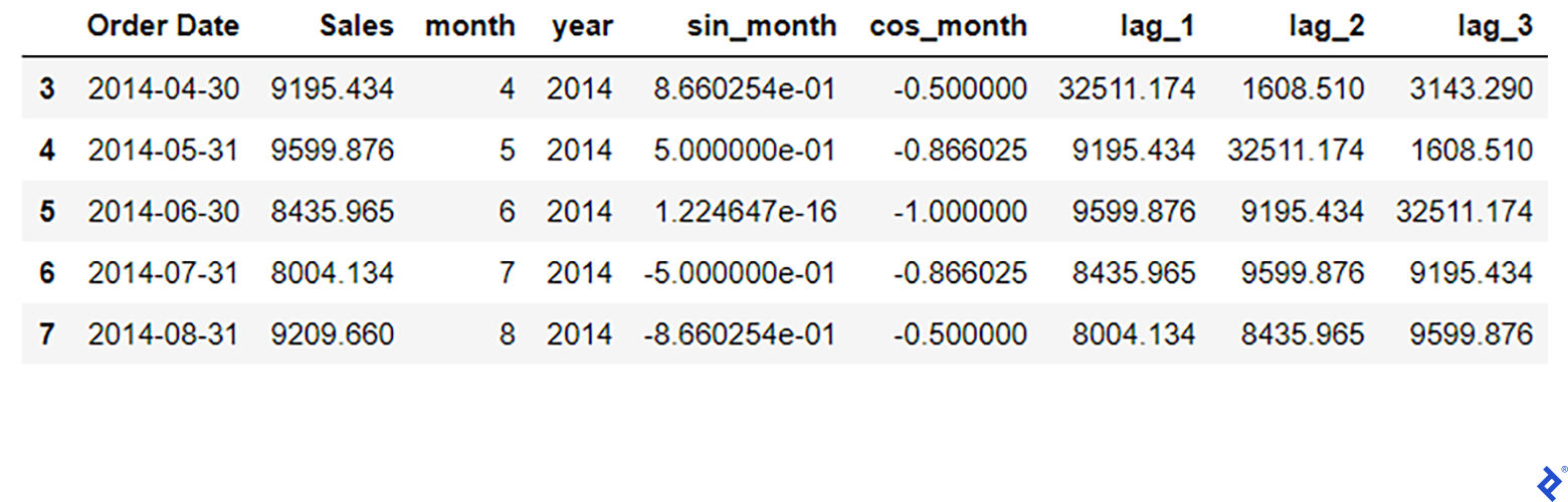
In this example, we’ve chosen a three-lag feature for our training set. This is a hyperparameter that can be determined using the autocorrelation plot or by experimenting with different values during the model tuning phase.

 1
 2
 3
 4
 5
 6
 7
 8
 9
10

X = df.drop(['Order Date','Sales'],axis = 1)
y = np.log1p(df['Sales'])


X_train,X_test,y_train,y_test = train_test_split(X,y,test_size = 0.2, shuffle=False)
y_pred = model.predict(X_test)

print(f'Loss with lag features on testing set is {sqrt(mean_squared_error(y_pred,y_test))}')

Loss with lag and aggregated sales features on testing set is 0.2862175857169188

By incorporating both lag features and cyclic conversions, our RMSE has further improved to 0.28.

Here are some more sales-related features you might want to consider:

• Item fraction sold (percentage of items sold relative to total store sales)
• Frequency of sales events for the item’s category
• Introducing the concept of “seniority”

Seniority helps categorize new items in a store:

• Seniority 0: Brand new items
• Seniority 1: Items sold in other branches but not in this particular store
• Seniority 2: Items previously sold in this store

Price-Related Features

Price, along with promotions, is a major driver of sales fluctuations. It’s also a key differentiator between product categories, subcategories, and super-categories.

For example, assuming each product has an assigned category and subcategory, we can engineer features like:

• (Mean, Max, Min, Median) prices within a category
• (Mean, Max, Min, Median) prices within a subcategory
• Comparisons between these statistics, such as the difference between each statistic in both the category and subcategory

We can perform this aggregation multiple times using different groupings based on the target period (e.g., monthly):

• Monthly, Store, category
• Monthly, Store, subcategory
• Monthly, Store, Item, category
• Monthly, Store, Item, subcategory

We can also exclude the Monthly grouping to analyze overall price behavior.

Stock-Related Features

While not as common, incorporating stock data can significantly enhance sales forecasting models. By combining daily inventory data for each product with sales data, we can calculate the monthly inventory turnover ratio, which indicates how quickly a product’s stock is sold. This ratio offers two main benefits:

• It helps the model forecast sales based on current inventory levels.
• It allows us to categorize products into slow-, medium-, and fast-moving groups, aiding in decision-making and modeling.

To calculate the inventory turnover ratio, you’ll need daily inventory and sales data:

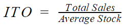
Note: These aggregations are performed over a specific timeframe. For monthly sales forecasting, the inventory turnover ratio would be calculated using the total sales and average inventory value for the same month.

Turning Sales Data into Opportunities

In conclusion, effective sales forecasting, driven by the right data pipelines and feature engineering techniques, can empower businesses to boost revenue and profitability. This article has shown how diverse data can be leveraged to achieve this.

Every company should assess whether AI can enhance its forecasting capabilities. If so, collaborating with skilled AI engineers and machine learning experts to develop a customized sales forecasting system is highly recommended.

For companies and retailers ready to embrace AI-powered sales forecasting, start by collecting as much data as possible, particularly daily sales, inventory, and transaction data.

Armed with this data, you can unlock significant revenue growth, optimize inventory replenishment strategies, and maximize profit potential, as demonstrated by the examples and best practices of leading retailers.

References:

The dataset Further reading on financial forecasting