Artificial intelligence (AI) is rapidly advancing, achieving remarkable performance in areas like image recognition, game playing, and even poker. This progress has generated excitement about the future possibilities of AI. However, there’s a growing concern about the unpredictable unreliability of AI in its current form.

A prime example is the Jeopardy! IBM Challenge, where IBM’s AI, Watson, dominated the game until the “Final Jeopardy!” round. The category was US Cities, and the clue was: “Its largest airport is named for a World War II hero; its second largest for a World War II battle.” Surprisingly, Watson answered, “What is Toronto?????”—the extra question marks (and low wager) indicating its doubt.

This illustrates a critical issue: while AI can perform exceptionally well for extended periods, it can still make unexpected and illogical errors. This unpredictability is a major obstacle to the widespread adoption of AI, particularly in safety-critical applications like self-driving cars.

This raises a crucial question: Can we develop AI models that make sound decisions even with incomplete information, ensuring reliability in critical situations? The answer, I believe, lies in monotonic machine learning models.

Without delving into technical details, monotonic AI models can address the limitations of current AI systems. With the right monotonic model:

• Self-driving cars would be safer, consistently prioritizing human safety signals.
• Machine learning (ML) systems would be more resilient to adversarial attacks and unforeseen circumstances.
• ML’s decision-making process would become more logical and understandable to humans.

We’re transitioning from an era of AI focused on computational power to one prioritizing effectiveness, understanding, and reliability. Monotonic machine learning models are at the forefront of this exciting shift.

Editor’s note: For a primer on ML fundamentals, readers can refer to our introductory ML article.

Understanding Monotonic AI Models

Simply put, a monotonic model is an ML model where the increase of certain features (monotonic features) always leads to an increase in the model’s output.

Real-world scenarios are replete with monotonic relationships:

• Gas prices rise with distance traveled.
• Loan approval chances improve with better credit scores.
• Driving time increases with traffic congestion.
• Revenue grows with ad click-through rates.

While these relationships seem obvious, an ML model working with limited data might not grasp them inherently, potentially leading to inaccurate predictions. Incorporating this inherent logic enhances an ML model’s performance, interpretability, and resistance to overfitting. In most cases, a monotonic model works best as part of a larger ensemble of learning models.

Monotonic AI models excel in adversarial robustness—they are difficult to deceive. Attackers limited to manipulating non-monotonic features cannot mislead the AI, as they can’t alter the example’s label in a way that affects the monotonic model’s output.

Real-world Applications of Monotonic AI Models

Let’s explore some practical applications of monotonic AI models:

Use Case #1: Malware Detection

Monotonic models play a crucial role in malware detection, as seen in Windows Defender. In one instance, malware creators fraudulently obtained trusted digital certificates to make their malicious software appear legitimate. A basic malware classifier relying on code-signing as a feature might misclassify such samples as safe.

However, Windows Defender’s monotonic model, trained on features exclusively indicative of malware, remains effective. Regardless of how malware creators disguise their software with benign elements, the monotonic model can still identify and neutralize the threat.

In my course, Machine Learning for Red Team Hackers, I demonstrate techniques to circumvent ML-based malware classifiers. One such technique involves padding malicious code with harmless content to evade detection by simplistic ML models. Monotonic models are resilient to such tactics, forcing attackers to exert significantly more effort to bypass them.

Use Case #2: Content Filtering

When developing content filters for sensitive environments like school libraries, monotonic models prove valuable. Inappropriate content might be present alongside a large volume of acceptable material.

A basic classifier might weigh “appropriate” features against “inappropriate” ones, potentially allowing access to harmful content if it constitutes a small proportion of the overall content. A monotonic model, however, can prioritize the presence of any inappropriate content as a critical factor, regardless of the volume of acceptable content.

Use Case #3: Self-driving Car AI

In the context of self-driving cars, consider an algorithm that detects a green light and a pedestrian simultaneously. A simple approach might weigh both signals equally. However, a pedestrian’s presence should always take precedence, regardless of the traffic signal.

Using a monotonic model with pedestrian presence as a monotonic feature ensures that the AI prioritizes safety and stops the car, even if other signals suggest proceeding.

Use Case #4: Recommendation Engines

Monotonic models benefit recommendation engines. These systems process numerous product attributes like star ratings, price, and review count. Assuming equal star ratings and prices, a product with more reviews is generally preferred. Monotonic models can enforce this logic, ensuring that higher review counts contribute positively to recommendations.

Use Case #5: Spam and Phishing Filtering

Similar to malware detection, spam and phishing filters can leverage monotonic models. Attackers often disguise malicious emails with seemingly harmless content to bypass filters. A monotonic model, however, can focus on features exclusively indicative of spam or phishing, rendering such disguises ineffective.

Implementation and Practical Examples

Several well-supported implementations of monotonic AI models are available, including XGBoost, LightGBM, and TensorFlow Lattice.

Monotonic ML XGBoost Tutorial

XGBoost is renowned for its performance in structured data analysis. It also supports monotonicity constraints.

The following XGBoost tutorial demonstrates how to use monotonic ML models, complete with an accompanying Python repo.

Begin by importing the necessary libraries:

1
2
3
4
5
6
7
8

import random
import numpy as np
import matplotlib.pyplot as plt
%matplotlib inline
from sklearn.metrics import confusion_matrix
import seaborn as sns

sns.set(font_scale=1.4)

This tutorial simulates a content filtering or malware detection scenario. We’ll use benign_features to represent factors like content related to “science,” “history,” or “sports” in content filtering or “code-signing” and “recognized authors” in malware detection. Conversely, malicious_features might represent content related to “violence” or “drugs” in content filtering or “calls to crypto libraries” and “similarity to known malware” in malware detection.

We’ll generate a dataset with a mix of benign and malicious samples, each with randomly generated features:

1
2
3

def flip():
    """Simulates a coin flip."""
    return 1 if random.random() < 0.5 else 0

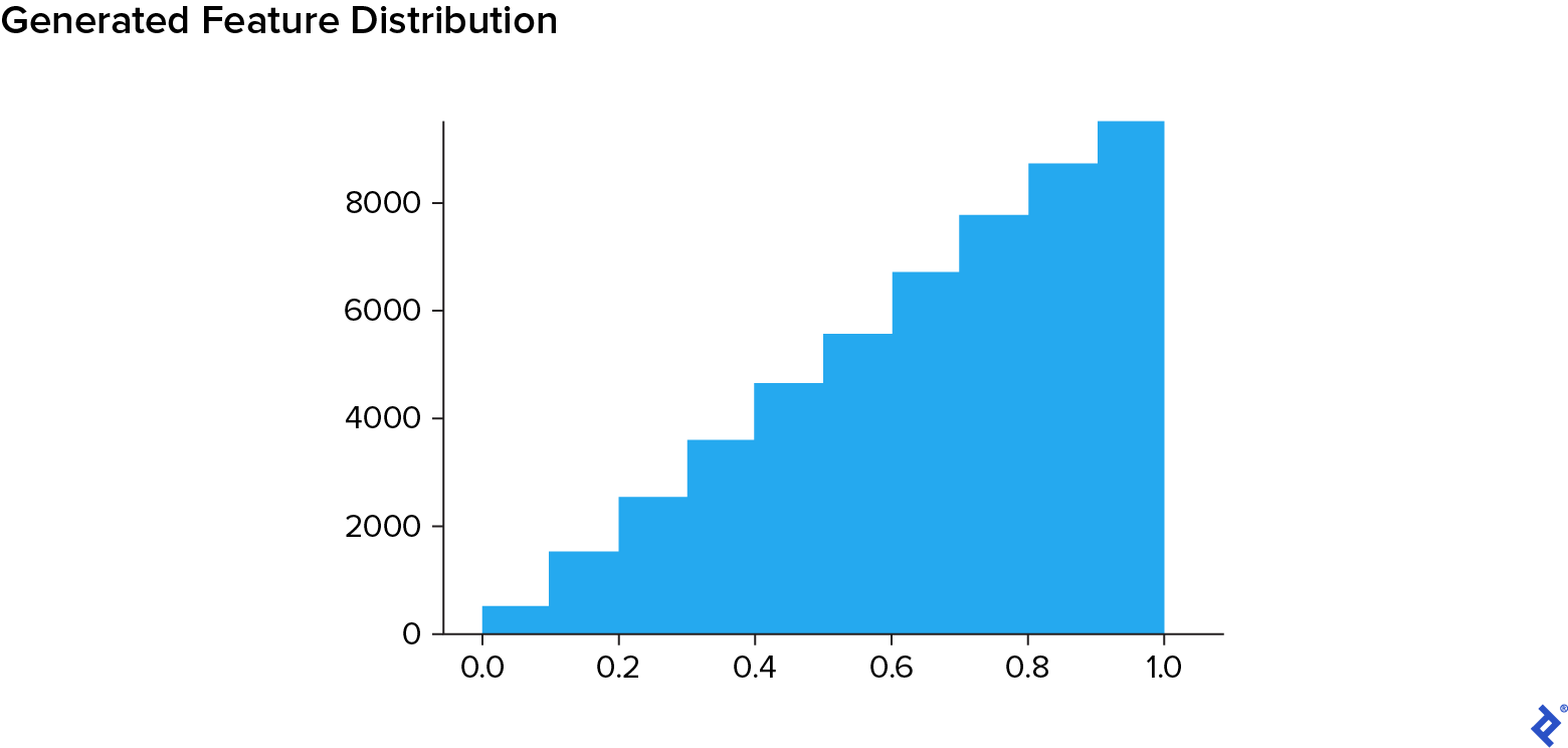
“Benign” samples will lean towards benign features, while “malicious” samples will favor malicious ones. We’ll use a triangular distribution to achieve this:

1
2
3

bins = [0.1 * i for i in range(12)]

plt.hist([random.triangular(0, 1, 1) for i in range(50000)], bins)

The following function captures this logic:

1
2
3

def generate():
    """Samples from the triangular distribution."""
    return random.triangular(0, 1, 1)

Next, we create our dataset:

 1
 2
 3
 4
 5
 6
 7
 8
 9
10
11
12
13
14
15
16
17
18
19
20
21
22

m = 100000
benign_features = 5
malicious_features = 5
n = benign_features + malicious_features
benign = 0
malicious = 1
X = np.zeros((m, n))
y = np.zeros((m))
for i in range(m):
    vec = np.zeros((n))
y[i] = flip()
if y[i] == benign:
    for j in range(benign_features):
        vec[j] = generate()
    for j in range(malicious_features):
        vec[j + benign_features] = 1 - generate()
else:
    for j in range(benign_features):
        vec[j] = 1 - generate()
    for j in range(malicious_features):
        vec[j + benign_features] = generate()
X[i, :] = vec

Here, X holds the randomly generated feature vectors, and y contains the corresponding labels. This classification problem is designed to be non-trivial.

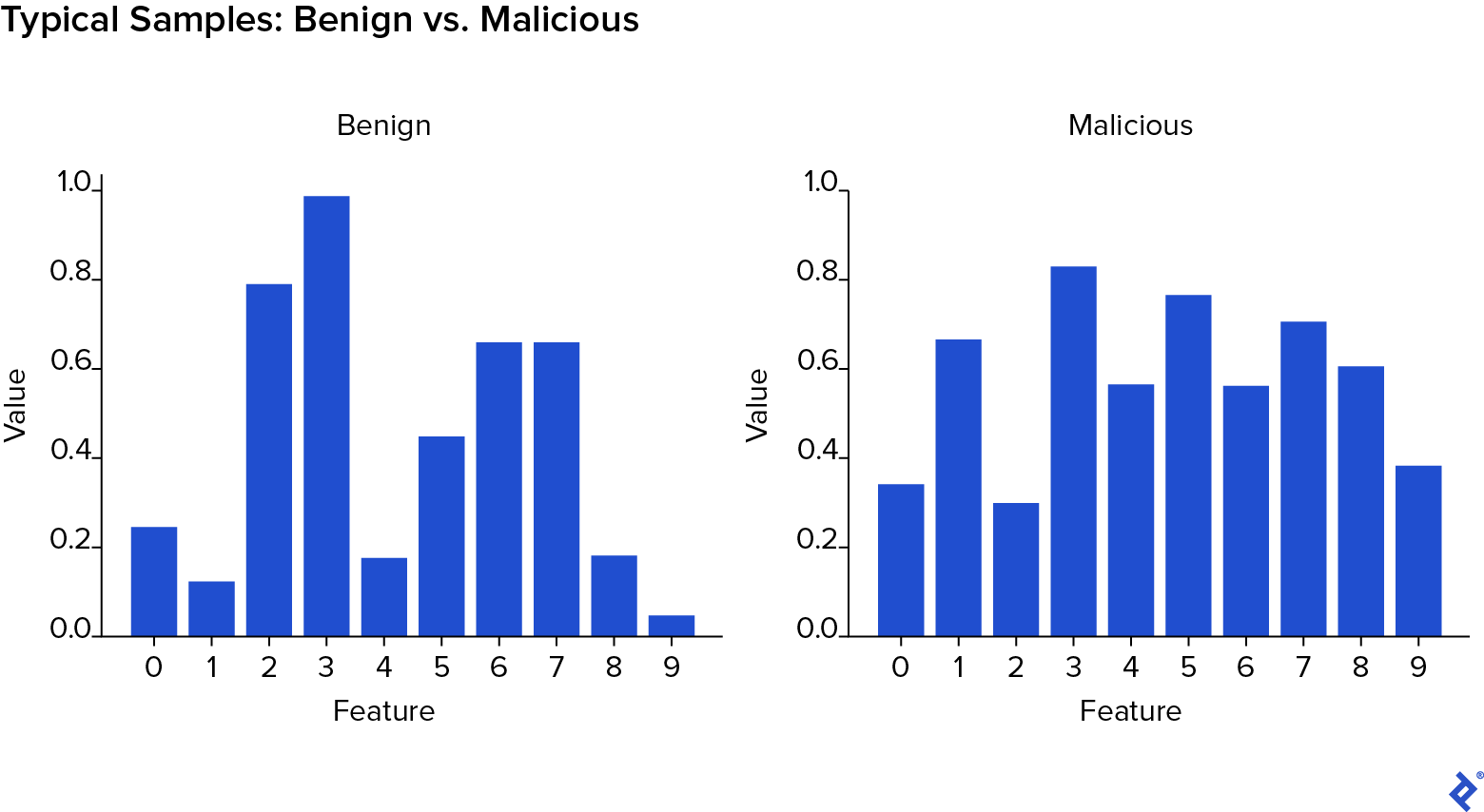
Observe that benign samples generally exhibit higher values in the initial features, while malicious samples have higher values in the later features.

We then split the data into training and testing sets:

1
2
3

from sklearn.model_selection import train_test_split

X_train, X_test, y_train, y_test = train_test_split(X, y, test_size=0.2)

The following function prepares the data for XGBoost:

1
2
3
4
5
6
7
8
9

import xgboost as xgb

def prepare_for_XGBoost(X, y):
    """Converts a numpy X and y dataset into a DMatrix for XGBoost."""
    return xgb.DMatrix(X, label=y)

dtrain = prepare_for_XGBoost(X_train, y_train)
dtest = prepare_for_XGBoost(X_test, y_test)
dall = prepare_for_XGBoost(X, y)

We first train and test a standard (non-monotonic) XGBoost model and evaluate its performance using a confusion matrix:

 1
 2
 3
 4
 5
 6
 7
 8
 9
10
11
12
13
14
15
16
17
18
19
20
21
22

params = {"n_jobs": -1, "tree_method": "hist"}
model_no_constraints = xgb.train(params=params, dtrain=dtrain)
CM = predict_with_XGBoost_and_return_confusion_matrix(
    model_no_constraints, dtrain, y_train
)
plt.figure(figsize=(12, 10))
sns.heatmap(CM / np.sum(CM), annot=True, fmt=".2%", cmap="Blues")
plt.ylabel("True Label")
plt.xlabel("Predicted Label")
plt.title("Unconstrained model's training confusion matrix")
plt.show()
print()
CM = predict_with_XGBoost_and_return_confusion_matrix(
    model_no_constraints, dtest, y_test
)
plt.figure(figsize=(12, 10))
sns.heatmap(CM / np.sum(CM), annot=True, fmt=".2%", cmap="Blues")
plt.ylabel("True Label")
plt.xlabel("Predicted Label")
plt.title("Unconstrained model's testing confusion matrix")
plt.show()
model_no_constraints = xgb.train(params=params, dtrain=dall)

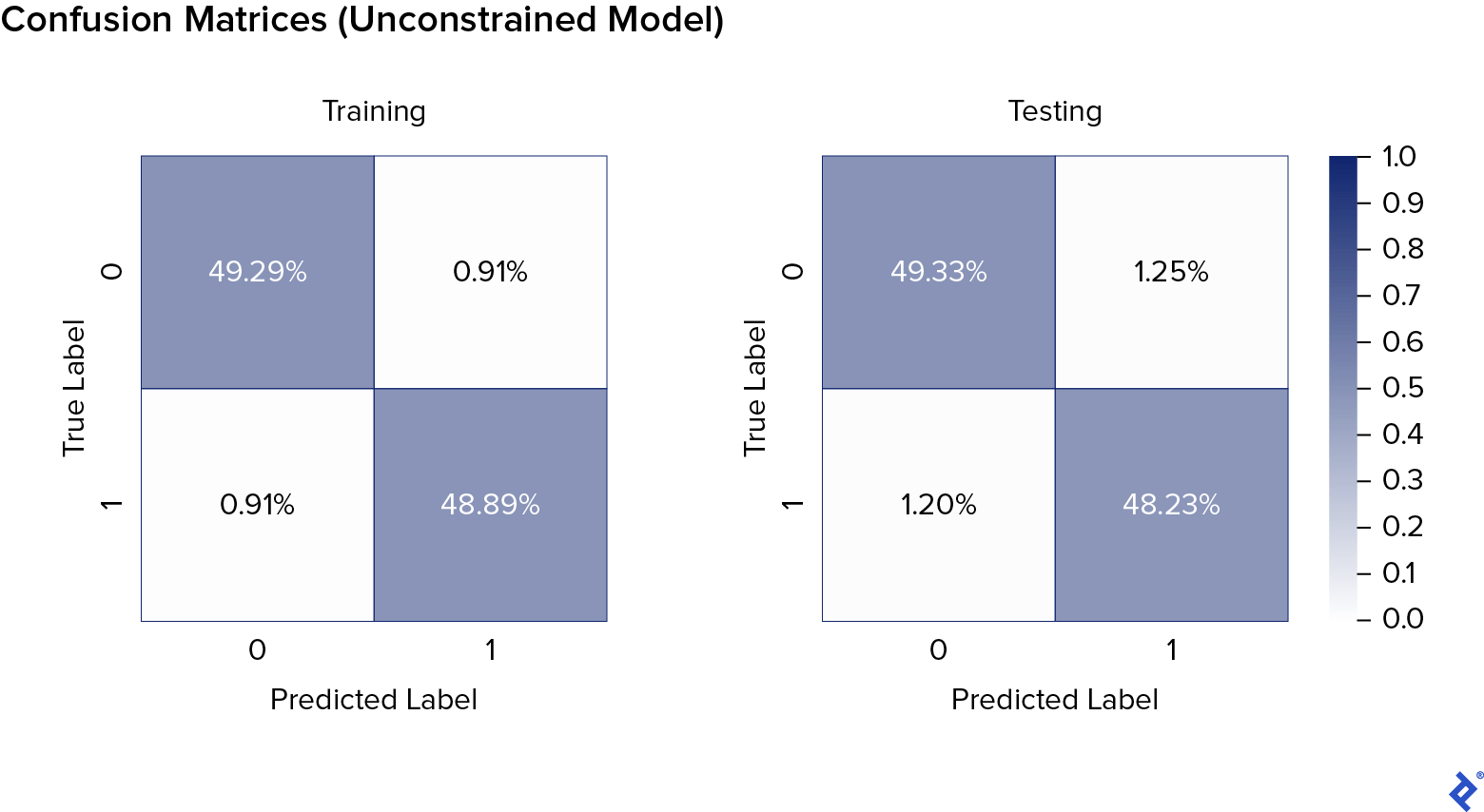
The results indicate no significant overfitting. We’ll compare this performance to monotonic models.

Now, let’s train and test a monotonic XGBoost model. We specify monotonicity constraints as a sequence (f0, f1, …, fN), where each fi is -1, 0, or 1, representing monotonically decreasing, unconstrained, or monotonically increasing features, respectively. In this case, we designate malicious features as monotonically increasing.

 1
 2
 3
 4
 5
 6
 7
 8
 9
10
11
12
13
14
15
16
17
18
19
20
21
22
23
24
25
26
27
28

params_constrained = params.copy()
monotone_constraints = (
    "("
    + ",".join([str(0) for m in range(benign_features)])
    + ","
    + ",".join([str(1) for m in range(malicious_features)])
    + ")"
)
print("Monotone constraints enforced are:")
print(monotone_constraints)
params_constrained["monotone_constraints"] = monotone_constraints
model_monotonic = xgb.train(params=params_constrained, dtrain=dtrain)
CM = predict_with_XGBoost_and_return_confusion_matrix(model_monotonic, dtrain, y_train)
plt.figure(figsize=(12, 10))
sns.heatmap(CM / np.sum(CM), annot=True, fmt=".2%", cmap="Blues")
plt.ylabel("True Label")
plt.xlabel("Predicted Label")
plt.title("Monotonic model's training confusion matrix")
plt.show()
print()
CM = predict_with_XGBoost_and_return_confusion_matrix(model_monotonic, dtest, y_test)
plt.figure(figsize=(12, 10))
sns.heatmap(CM / np.sum(CM), annot=True, fmt=".2%", cmap="Blues")
plt.ylabel("True Label")
plt.xlabel("Predicted Label")
plt.title("Monotonic model's testing confusion matrix")
plt.show()
model_monotonic = xgb.train(params=params_constrained, dtrain=dall)

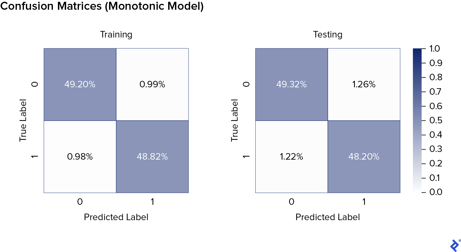
The monotonic model exhibits similar performance to the unconstrained model.

To further test robustness, we’ll create an adversarial dataset by manipulating the malicious samples to appear more benign:

1
2
3
4
5
6
7

X_adversarial = X[y == malicious]
y_adversarial = len(X_adversarial) * [malicious]
for i in range(len(X_adversarial)):
    vec = X_adversarial[i, :]
    for j in range(benign_features):
        vec[j] = 1
    X_adversarial[i, :] = vec

We then format this adversarial data for XGBoost:

1

dadv = prepare_for_XGBoost(X_adversarial, y_adversarial)

Finally, we test both models on the adversarial dataset:

1
2
3
4
5
6
7
8
9

CM = predict_with_XGBoost_and_return_confusion_matrix(
    model_no_constraints, dadv, y_adversarial
)
plt.figure(figsize=(12, 10))
sns.heatmap(CM / np.sum(CM), annot=True, fmt=".2%", cmap="Blues")
plt.ylabel("True Label")
plt.xlabel("Predicted Label")
plt.title("Unconstrained model's confusion matrix on adversarial dataset")
plt.show()

1
2
3
4
5
6
7
8
9

CM = predict_with_XGBoost_and_return_confusion_matrix(
    model_monotonic, dadv, y_adversarial
)
plt.figure(figsize=(12, 10))
sns.heatmap(CM / np.sum(CM), annot=True, fmt=".2%", cmap="Blues")
plt.ylabel("True Label")
plt.xlabel("Predicted Label")
plt.title("Monotonic model's confusion matrix on adversarial dataset")
plt.show()

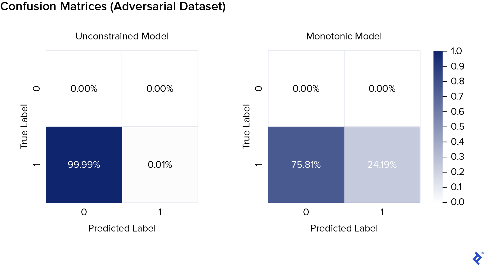
The results demonstrate the monotonic model’s significantly higher resistance to adversarial attacks.

LightGBM

LightGBM offers a similar approach to implementing monotonic constraints. is similar provides the syntax.

TensorFlow Lattice

TensorFlow Lattice provides pre-built TensorFlow Estimators and operators for creating lattice models—multi-dimensional interpolated look-up tables. As described in the Google AI Blog:

“…look-up table values are trained to minimize loss on training examples, with adjacent values constrained to increase along specific input dimensions, ensuring output increases in those directions. Interpolation between look-up table values ensures smooth predictions and avoids extreme values during testing.”

Tutorials for utilizing TensorFlow Lattice can be found here.

Monotonic AI: Shaping the Future

Monotonic AI models have emerged as a valuable tool, enhancing security, providing logical recommendations, and fostering greater trust in AI systems. They mark a significant step towards a future where AI is characterized by safety, reliability, and understandability. As we delve deeper into this exciting realm, monotonic models hold the key to unlocking the full potential of AI while mitigating its risks.