In the realm of traditional programming, programmers meticulously craft each software instruction, leaving no room for learning from data. Conversely, machine learning, a fascinating branch of computer science, empowers computers to learn and extract knowledge from data using statistical methods, without the need for explicit programming.

This reinforcement learning tutorial will demonstrate how to utilize PyTorch to train a reinforcement learning neural network to master the game Flappy Bird. Before delving into the implementation, let’s establish a foundation by exploring some essential building blocks.

Machine learning algorithms can be broadly categorized into two groups: traditional learning algorithms and deep learning algorithms. Traditional learning algorithms, typically characterized by fewer learnable parameters, possess a limited learning capacity compared to their deep learning counterparts.

Furthermore, traditional learning algorithms lack the ability to perform feature extraction. This limitation necessitates artificial intelligence specialists to meticulously design a suitable data representation, which is then fed into the learning algorithm. Examples of traditional machine learning techniques include SVM, random forest, decision tree, and $k$-means. In contrast, the deep neural network takes center stage as the central algorithm in deep learning.

Deep neural networks excel in their ability to process raw data, such as images, directly, eliminating the need for artificial intelligence specialists to handcraft data representations. Instead, the neural network autonomously discovers the optimal representation during the training process.

While many deep learning techniques have existed for a considerable time, recent hardware advancements, particularly in the realm of GPUs spearheaded by Nvidia, have significantly accelerated deep learning research and development, enabling rapid experimentation.

Learnable Parameters and Hyperparameters

Machine learning algorithms comprise two types of parameters: learnable parameters, which are fine-tuned during the training process, and non-learnable parameters, which are predetermined before training. These pre-set parameters are referred to as hyperparameters.

Grid search stands as a widely employed method for determining the optimal hyperparameters. This brute-force technique involves exhaustively evaluating all possible hyperparameter combinations within a defined range and selecting the combination that maximizes a predefined metric.

Supervised, Unsupervised, and Reinforcement Learning Algorithms

One approach to classifying learning algorithms is to differentiate between supervised and unsupervised algorithms. However, it’s important to note that reinforcement learning exists on a spectrum between these two categories.

In supervised learning, we deal with $ (x_i, y_i) $ pairs, where $ x_i $ represents the input to the algorithm and $ y_i $ represents the desired output. The objective is to identify a function that accurately maps $ x_i $ to $ y_i $.

To optimize the learnable parameters and establish a function that effectively maps $ x_i $ to $ y_i $, a loss function and an optimizer are required. The optimizer’s role is to minimize the loss function. A commonly used loss function is the mean squared error (MSE):

[MSE = \sum_{i=1}^{n} (y_i - \widehat{y_i} )^2]

In this equation, $ y_i $ represents the ground truth label, while $ \widehat{y_i} $ denotes the predicted label. Stochastic gradient descent has gained significant popularity as an optimizer in deep learning. Numerous variations, such as Adam, Adadelta, and Adagrad, strive to enhance the performance of stochastic gradient descent.

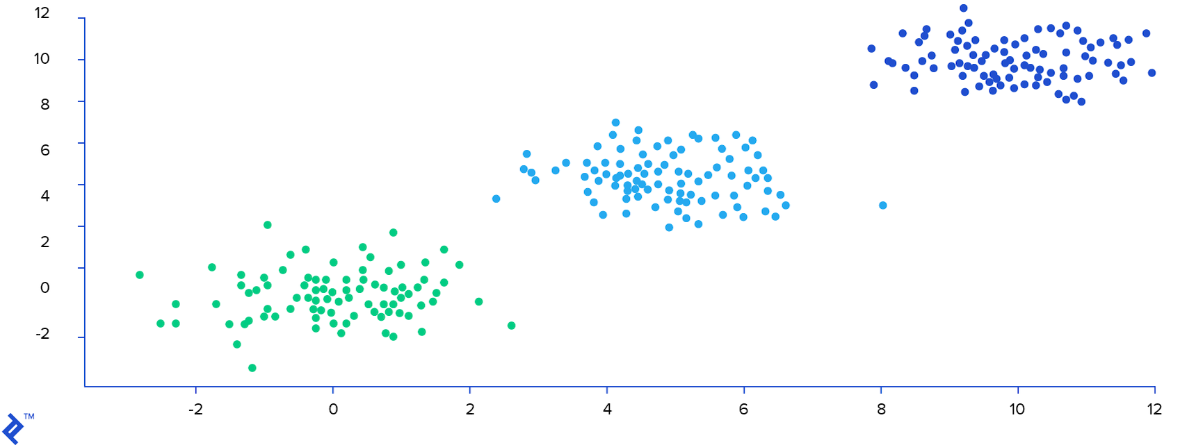
Unsupervised algorithms, on the other hand, aim to uncover underlying structures within data without relying on explicit labels. One such algorithm is $k$-means, which seeks to identify optimal clusters within a dataset. To illustrate, consider an image comprising 300 data points. The $k$-means algorithm successfully identifies the inherent structure in the data and assigns a cluster label, represented by a distinct color, to each data point.

Reinforcement learning distinguishes itself through the use of rewards - sparse, time-delayed labels. An agent interacts with its environment by taking actions, which in turn alter the environment’s state. Based on these actions, the agent receives new observations and rewards. Observations represent the stimuli that the agent perceives from the environment, encompassing sights, sounds, smells, and more.

Rewards are presented to the agent upon taking actions, serving as indicators of the action’s effectiveness. Through the process of perceiving observations and rewards, the agent progressively learns how to navigate and interact optimally within its environment. We will explore this concept in greater detail shortly.

Active, Passive, and Inverse Reinforcement Learning

Within the realm of reinforcement learning, several distinct approaches exist. In this tutorial, we focus on active reinforcement learning, where the agent actively interacts with the environment to learn. In contrast, passive reinforcement learning treats rewards merely as additional observations, with decisions being made based on a predetermined fixed policy.

Inverse reinforcement learning takes a different route by attempting to reconstruct the reward function given a history of actions and their corresponding rewards in various states.

Generalization, Overfitting, and Underfitting

In machine learning, a specific configuration of parameters and hyperparameters is referred to as a model. Machine learning experiments generally consist of two phases: training and testing.

During training, learnable parameters are adjusted using a training dataset. In the testing phase, these parameters are frozen, and the model’s performance is evaluated based on its ability to make accurate predictions on unseen data. Generalization refers to the model’s capacity to perform well on novel, previously unencountered examples or tasks after being trained on a specific dataset.

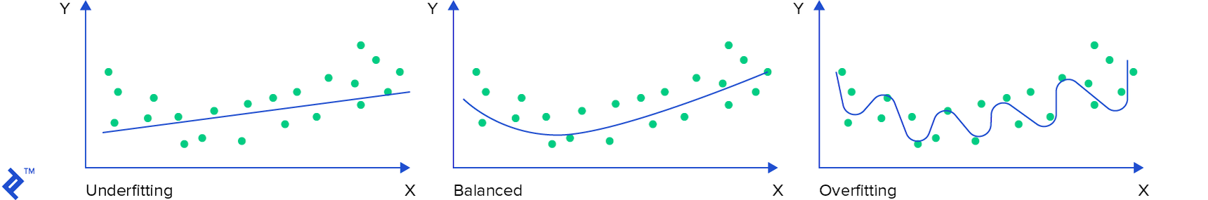
If a model is overly simplistic relative to the complexity of the data, it may struggle to fit the training data adequately, leading to poor performance on both the training and test datasets. This phenomenon is known as underfitting.

Conversely, when a model exhibits excellent performance on the training data but performs poorly on the test data, it is indicative of overfitting. Overfitting occurs when a model becomes overly tailored to the training data, failing to generalize well to unseen examples.

The following image illustrates the concepts of underfitting and overfitting in comparison to a balanced scenario where the prediction function aligns well with the overall data distribution.

Scalability

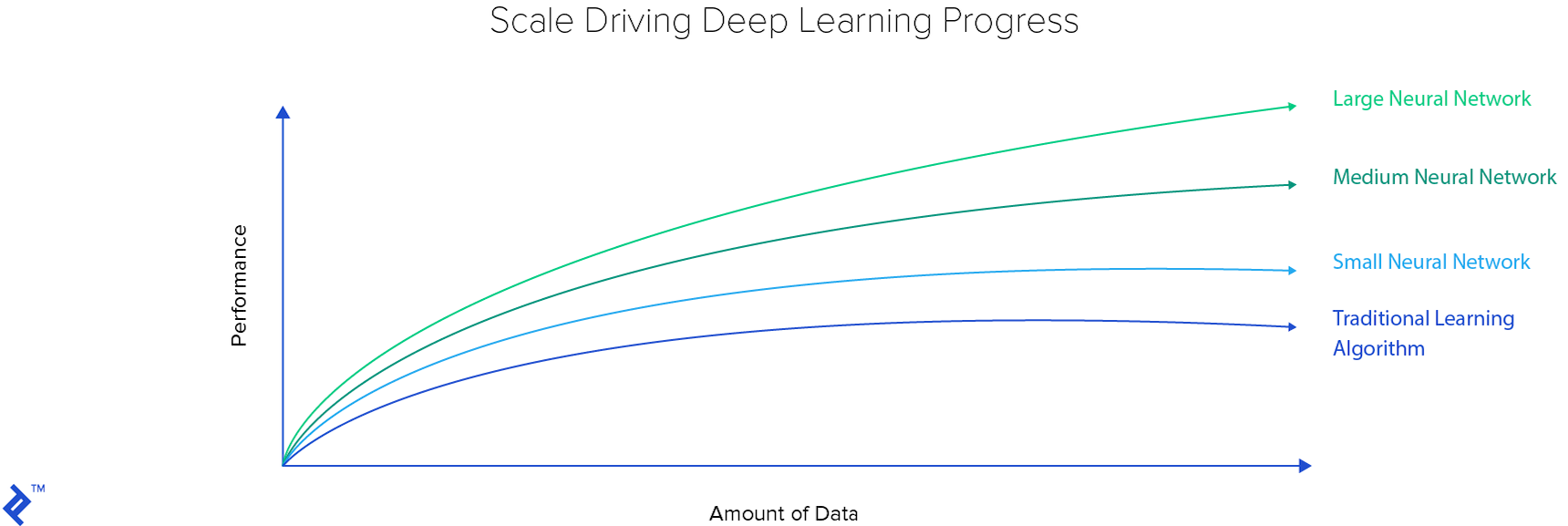
Data plays a pivotal role in the development of robust machine learning models. While traditional learning algorithms may not necessitate extensive datasets, their limited capacity often translates to restricted performance. The accompanying plot highlights the superior scalability of deep learning methods compared to their traditional counterparts.

Neural Networks

Neural networks are sophisticated structures composed of interconnected layers. A simplified representation of a four-layered neural network is depicted in the image below. The first layer acts as the input layer, responsible for receiving input data, while the last layer serves as the output layer, producing the final output. Sandwiched between the input and output layers are two hidden layers responsible for intermediate computations.

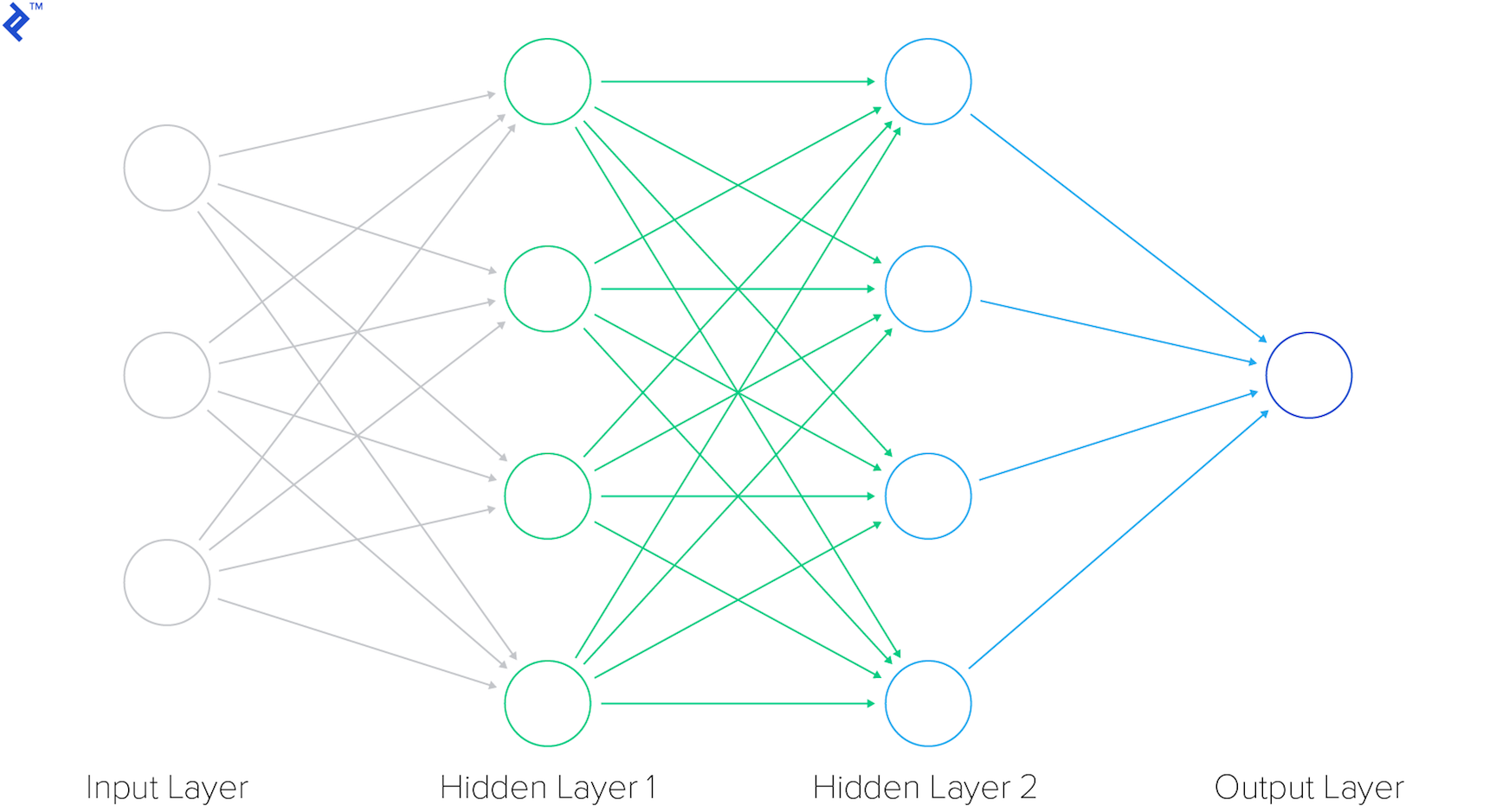
Neural networks containing more than one hidden layer are categorized as deep neural networks. Given an input set $ X $, the neural network processes the data and generates an output $ y $. The learning process unfolds through the backpropagation algorithm, which leverages a loss function and an optimizer.

Backpropagation comprises two key steps: a forward pass and a backward pass. In the forward pass, input data is fed into the neural network, producing an output. The discrepancy between the ground truth and the prediction is quantified as a loss. Subsequently, during the backward pass, the neural network’s parameters are adjusted based on the calculated loss to improve accuracy.

Convolutional Neural Network

A notable variation of the neural network architecture is the convolutional neural network, particularly well-suited for computer vision tasks.

The convolutional layer, from which the network derives its name, stands as the most crucial component of a convolutional neural network. This layer’s parameters consist of learnable filters, often referred to as kernels. Convolutional layers apply convolution operations to the input, effectively reducing the number of learnable parameters. This reduction acts as a form of heuristics, simplifying the neural network’s training process and enhancing its efficiency.

The following illustration demonstrates the operation of a single convolutional kernel within a convolutional layer. The kernel slides across the input image, performing element-wise multiplications and summations to produce a convolved feature map.

ReLU (Rectified Linear Unit) layers play a critical role in introducing non-linearities into the neural network. Non-linearities are essential because they empower the network to model a wide range of functions, extending beyond linear relationships. The ReLU function is defined as follows:

[ReLU = \max(0, x)]

In essence, the ReLU function acts as a threshold, effectively suppressing negative values to zero.

[ReLU = \max(0, x)]

ReLU is one of many activation functions employed to incorporate non-linearities into neural networks. Other examples include sigmoid and hyperbolic tangent functions. ReLU’s popularity stems from its ability to facilitate efficient neural network training compared to its alternatives.

The plot below visually represents the ReLU function.

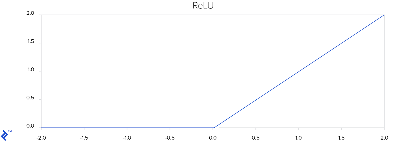
As the plot illustrates, the ReLU function effectively rectifies negative values to zero. This helps prevent the vanishing gradient problem. If a gradient vanishes during training, it will have a negligible impact on adjusting the neural network’s weights.

Convolutional neural networks typically comprise a combination of convolutional layers, ReLU layers, and fully connected layers. Fully connected layers establish connections between every neuron in one layer and every neuron in the subsequent layer, as observed in the two hidden layers depicted in the initial neural network image. The final fully connected layer maps the outputs from the preceding layer to a desired number of outputs, which in this case corresponds to the number_of_actions.

Applications

Deep learning has demonstrated remarkable success and consistently outperforms classical machine learning algorithms across various subfields, including computer vision, speech recognition, and reinforcement learning. These deep learning advancements have found practical applications in diverse real-world domains, spanning finance, medicine, entertainment, and more.

Reinforcement Learning

At the heart of reinforcement learning lies the concept of an agent. An agent interacts with its environment by taking actions, receiving observations, and obtaining rewards in return. The primary objective of training an agent is to maximize its cumulative reward.

Unlike classical machine learning algorithms, where machine learning engineers bear the responsibility of feature extraction, deep learning empowers the creation of end-to-end systems. These systems can process high-dimensional inputs, such as video streams, and autonomously learn optimal strategies for agents to make informed decisions.

In 2013, DeepMind, an AI startup based in London, achieved a significant breakthrough in training agents directly from high-dimensional sensory inputs. Their seminal paper, Playing Atari with Deep Reinforcement Learning, showcased their success in teaching an artificial neural network to master Atari games by solely observing the screen. Following their acquisition by Google, DeepMind further refined their approach and published an updated paper in Nature: Human-level control through deep reinforcement learning.

Reinforcement learning stands apart from other machine learning paradigms by eschewing the need for a direct supervisor. Instead, it relies solely on a reward signal to guide the agent’s learning process. Feedback is inherently delayed, unlike the instantaneous feedback mechanisms employed in supervised learning algorithms. Additionally, data in reinforcement learning is sequential, with the agent’s actions influencing the subsequent data it receives.

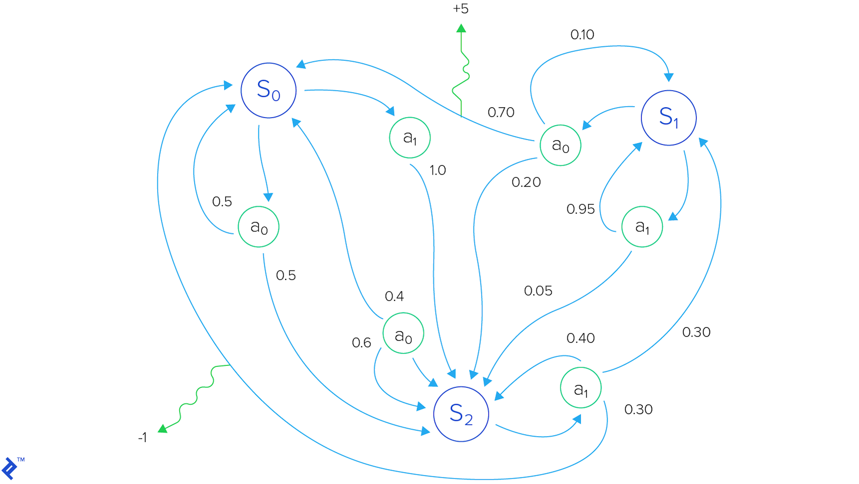
To formalize the agent’s interaction with the environment, we employ the framework of a Markov decision process, which a formal way of modeling this reinforcement learning environment. This mathematical framework comprises a set of states, a set of available actions, and rules (e.g., probabilities) that govern transitions between states.

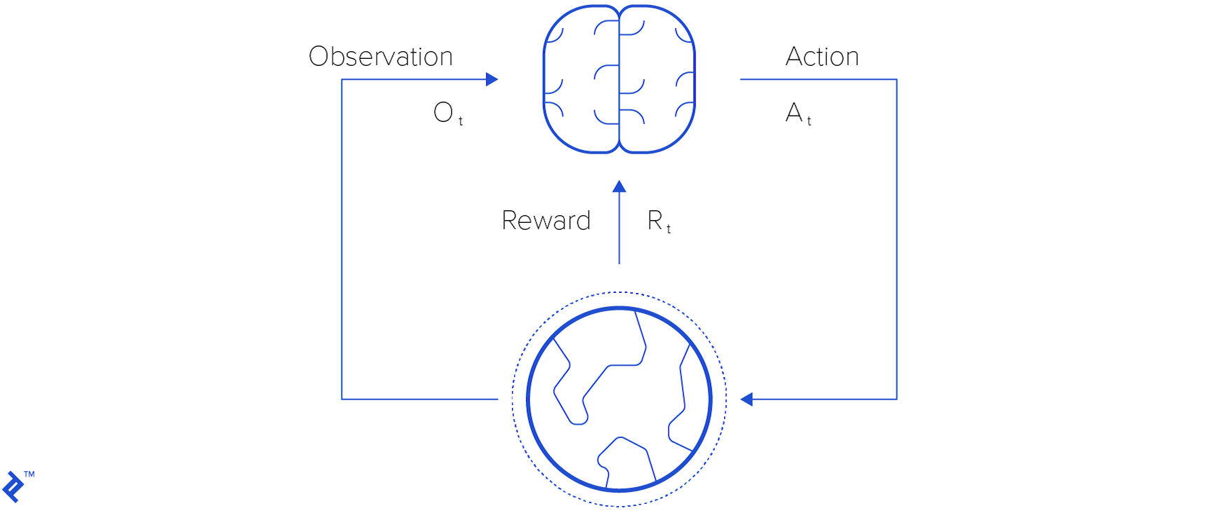
The agent possesses the ability to execute actions, thereby altering the environment’s state. The outcome of these actions is reflected in the reward, denoted as $ R_t $, a scalar feedback signal indicating the agent’s performance at a given time step $t$.

Optimizing for long-term performance necessitates considering not only immediate rewards but also future rewards. The total reward for a single episode starting from time step $t$ is given by $ R_t = r_t + r_{t+1} + r_{t+2} + \ldots + r_n $. However, due to the inherent uncertainty of future predictions, a discounted future reward is employed: $ R_t = r_t +\gamma r_{t+1} + \gamma^2r_{t+2} + \ldots + \gamma^{n-t}r_n = r_t + \gamma R_{t+1} $. Here, $ \gamma $ represents a discount factor that diminishes the significance of rewards as they extend further into the future. The agent’s goal is to select actions that maximize this discounted future reward.

Deep Q-learning

The $ Q(s, a) $ function, central to deep Q-learning, quantifies the maximum discounted future reward attainable when action $ a $ is executed in state $ s $:

[Q(s_t, a_t) = \max R_{t+1}]

The Bellman equation provides a recursive relationship for estimating future rewards: $ Q(s, a) = r + \gamma \max_{a’}Q(s’, a’) $. This equation states that the maximum future reward, given a state $ s $ and action $ a $, is equivalent to the immediate reward plus the maximum future reward attainable from the subsequent state $ s’ $ after taking the optimal action $ a’ $.

Directly approximating Q-values using non-linear functions, such as neural networks, can introduce instability into the learning process. To mitigate this, experience replay is employed. Experience replay involves storing the agent’s experiences (state transitions, actions, rewards) during training episodes in a replay memory. Instead of utilizing only the most recent transition, random mini-batches are sampled from the replay memory. This sampling technique disrupts the correlation between consecutive training samples, preventing the neural network from converging to suboptimal local minima.

Two crucial aspects of deep Q-learning warrant attention: exploration and exploitation. Exploitation entails making the best decision based on the currently available information, while exploration focuses on gathering more information to potentially discover better actions.

When the algorithm chooses actions based on the neural network’s recommendations, it is said to be exploiting the network’s learned knowledge. Conversely, when the algorithm opts for random actions, it is exploring new possibilities, potentially enriching the neural network’s knowledge base.

The following excerpt from DeepMind’s paper Playing Atari with Deep Reinforcement Learning outlines the “Deep Q-learning algorithm with Experience Replay”:

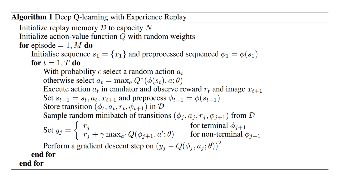
DeepMind coined the term Deep Q-networks (DQN) to refer to convolutional networks trained using their proposed deep Q-learning approach.

Deep Q-learning Example Using Flappy Bird

Flappy Bird, a mobile game that took the world by storm, was the brainchild of Vietnamese video game artist and programmer Dong Nguyen. In this deceptively simple yet challenging game, the player assumes control of a bird, navigating it through a series of green pipes without colliding with them.

A screenshot from a Flappy Bird clone coded using PyGame is provided below for reference:

Since its inception, the original Flappy Bird game has been cloned, modified, and adapted for various purposes. One such modification, which we’ll be using in this tutorial, strips away the background, sounds, and different bird and pipe styles, focusing solely on the core game mechanics. This modified game engine is sourced from this TensorFlow project:

However, instead of relying on TensorFlow, the deep reinforcement learning framework in this tutorial is built using PyTorch. PyTorch, known for its speed and flexibility, provides a powerful platform for deep learning experimentation, offering tensors, dynamic neural networks in Python, and robust GPU acceleration.

The neural network architecture employed in this tutorial mirrors the one used by DeepMind in their paper Human-level control through deep reinforcement learning.

The network consists of three convolutional layers followed by two fully connected layers. ReLU activation is applied to each layer except the last, which utilizes linear activation. The network’s output comprises two values, representing the two possible actions available to the player: “Fly up” and “Do nothing.”

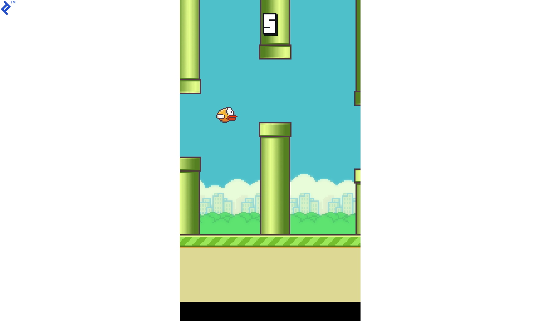
The input to the network consists of four consecutive 84x84 grayscale images. An example of four such images, which would be fed to the neural network, is shown below.

You’ll observe that the images are rotated. This rotation stems from the output format of the modified game engine. However, this rotation does not hinder the neural network’s performance during training or testing.

Furthermore, the images are cropped to exclude the floor, as it is irrelevant to the task at hand. Pixels representing the pipes and the bird are white, while background pixels are black.

The following code snippet showcases the definition of the neural network. The network’s weights are initialized using a uniform distribution $\mathcal{U}(-0.01, 0.01)$, while the bias terms are set to 0.01. Although various weight initializations Several different initializations were explored, including Xavier uniform, Xavier normal, Kaiming uniform, Kaiming normal, uniform, and normal, the chosen initialization proved to result in the fastest convergence and training time for this particular task. The size of the neural network is 6.8 MB.

 1
 2
 3
 4
 5
 6
 7
 8
 9
10
11
12
13
14
15
16
17
18
19
20
21
22
23
24
25
26
27
28
29
30
31
32
33
34
35
36

class NeuralNetwork(nn.Module):

    def __init__(self):
        super(NeuralNetwork, self).__init__()

        self.number_of_actions = 2
        self.gamma = 0.99
        self.final_epsilon = 0.0001
        self.initial_epsilon = 0.1
        self.number_of_iterations = 2000000
        self.replay_memory_size = 10000
        self.minibatch_size = 32

        self.conv1 = nn.Conv2d(4, 32, 8, 4)
        self.relu1 = nn.ReLU(inplace=True)
        self.conv2 = nn.Conv2d(32, 64, 4, 2)
        self.relu2 = nn.ReLU(inplace=True)
        self.conv3 = nn.Conv2d(64, 64, 3, 1)
        self.relu3 = nn.ReLU(inplace=True)
        self.fc4 = nn.Linear(3136, 512)
        self.relu4 = nn.ReLU(inplace=True)
        self.fc5 = nn.Linear(512, self.number_of_actions)

    def forward(self, x):
        out = self.conv1(x)
        out = self.relu1(out)
        out = self.conv2(out)
        out = self.relu2(out)
        out = self.conv3(out)
        out = self.relu3(out)
        out = out.view(out.size()[0], -1)
        out = self.fc4(out)
        out = self.relu4(out)
        out = self.fc5(out)

        return out

Within the constructor, you’ll notice the definition of hyperparameters. Hyperparameter optimization is not performed in this particular blog post. Instead, the hyperparameter values are largely adopted from DeepMind’s papers, with some adjustments made to suit the complexity of Flappy Bird compared to the Atari games used in their research.

Specifically, the epsilon value, which governs the exploration-exploitation trade-off, is significantly reduced compared to DeepMind’s paper. DeepMind uses an epsilon of one, while this implementation utilizes a value of 0.1. This reduction is motivated by the observation that higher epsilon values lead to excessive flapping, often resulting in the bird colliding with the upper screen boundary.

The reinforcement learning code operates in two modes: training and testing. During testing, the algorithm’s performance is evaluated to assess how effectively it has learned to play the game. However, before testing, the neural network must first be trained. This involves defining a loss function to minimize and an optimizer to guide the minimization process. In this implementation, the Adam optimization algorithm is employed in conjunction with the mean squared error loss function:

1
2

optimizer = optim.Adam(model.parameters(), lr=1e-6)
criterion = nn.MSELoss()

Next, an instance of the game is created:

1

game_state = GameState()

A Python list is used to implement the replay memory:

1

replay_memory = []

The initial state is then initialized. Actions are represented as two-dimensional tensors:

• [1, 0] corresponds to the “Do nothing” action.
• [0, 1] corresponds to the “Fly up” action.

The frame_step method provides the next game screen, the reward obtained, and a boolean flag indicating whether the current state is terminal (game over). A reward of 0.1 is awarded for each move the bird makes without crashing, as long as it is not passing through a pipe. Successfully passing through a pipe grants a reward of 1, while crashing results in a penalty of -1.

The resize_and_bgr2gray function handles cropping the floor, resizing the game screen to an 84x84 image, and converting the color space from BGR to grayscale. The image_to_tensor function converts the processed image to a PyTorch tensor and transfers it to GPU memory if CUDA is available. Finally, the last four consecutive screens are concatenated to create the input for the neural network.

1
2
3
4
5
6

action = torch.zeros([model.number_of_actions], dtype=torch.float32)
action[0] = 1
image_data, reward, terminal = game_state.frame_step(action)
image_data = resize_and_bgr2gray(image_data)
image_data = image_to_tensor(image_data)
state = torch.cat((image_data, image_data, image_data, image_data)).unsqueeze(0)

The initial epsilon value is set as follows:

1

epsilon = model.initial_epsilon

The core training loop is then executed. Comments embedded within the code provide insights into its operation, and you can compare it to the Deep Q-learning with Experience Replay algorithm described earlier.

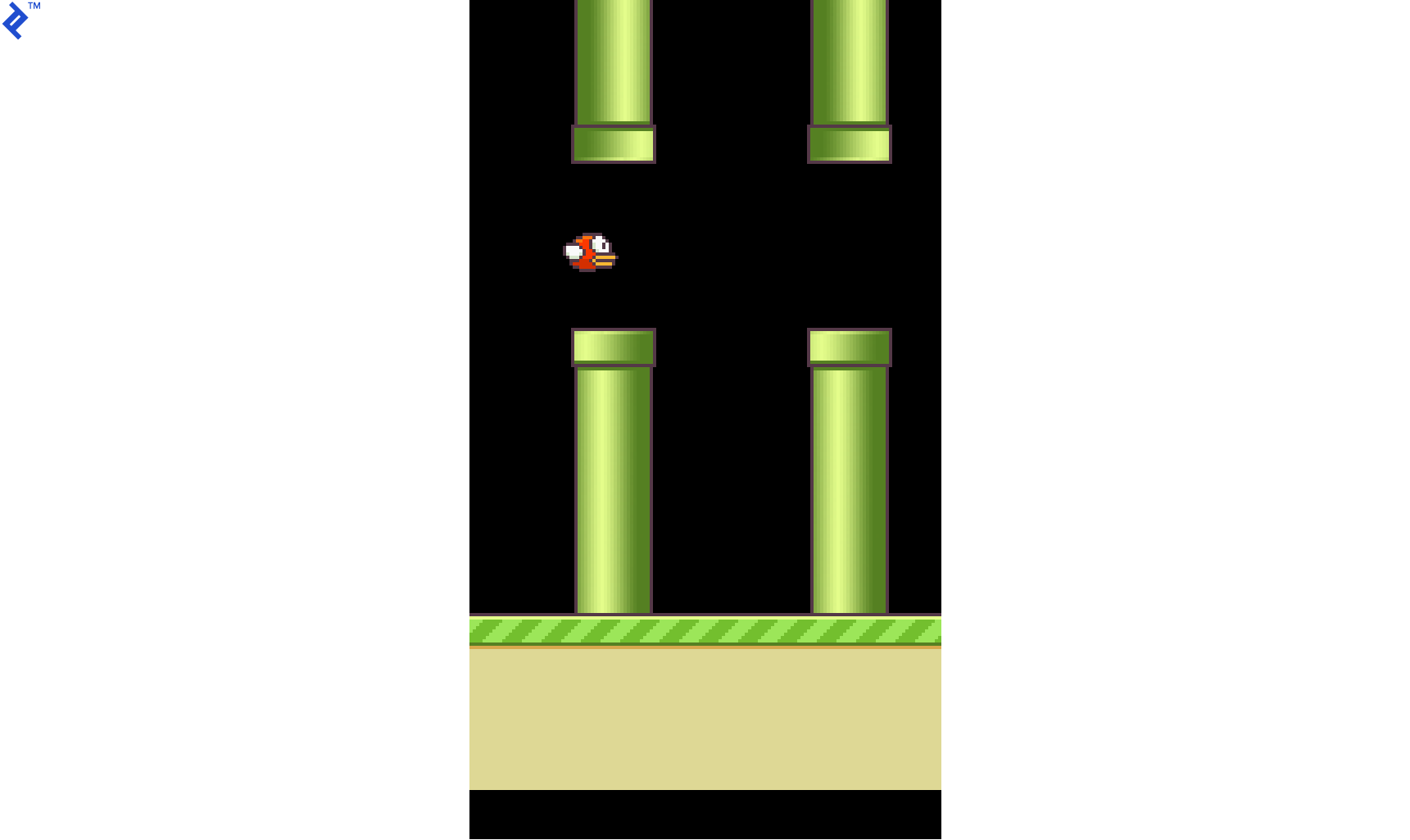
The algorithm samples mini-batches of experiences from the replay memory and updates the neural network’s parameters accordingly. Actions are chosen using an epsilon-greedy exploration strategy, where epsilon annealed over time. The loss function being minimized is $ L = \frac{1}{2}\left[\max_{a’}Q(s’, a’) - Q(s, a)\right]^2 $. $ Q(s, a) $ represents the target Q-value calculated using the Bellman equation, while $ \max_{a’}Q(s’, a’) $ is the predicted Q-value obtained from the neural network. The neural network outputs two Q-values, one for each possible action, and the algorithm selects the action associated with the higher Q-value.

 1
 2
 3
 4
 5
 6
 7
 8
 9
10
11
12
13
14
15
16
17
18
19
20
21
22
23
24
25
26
27
28
29
30
31
32
33
34
35
36
37
38
39
40
41
42
43
44
45
46
47
48
49
50
51
52
53
54
55
56
57
58
59
60
61
62
63
64
65
66
67
68
69
70
71
72
73
74
75
76
77
78
79
80
81
82

while iteration < model.number_of_iterations:
    # get output from the neural network
    output = model(state)[0]

    # initialize action
    action = torch.zeros([model.number_of_actions], dtype=torch.float32)
    if torch.cuda.is_available():  # put on GPU if CUDA is available
        action = action.cuda()

    # epsilon greedy exploration
    random_action = random.random() <= epsilon
    if random_action:
        print("Performed random action!")
    action_index = [torch.randint(model.number_of_actions, torch.Size([]), dtype=torch.int)
                    if random_action
                    else torch.argmax(output)][0]

    if torch.cuda.is_available():  # put on GPU if CUDA is available
        action_index = action_index.cuda()

    action[action_index] = 1

    # get next state and reward
    image_data_1, reward, terminal = game_state.frame_step(action)
    image_data_1 = resize_and_bgr2gray(image_data_1)
    image_data_1 = image_to_tensor(image_data_1)
    state_1 = torch.cat((state.squeeze(0)[1:, :, :], image_data_1)).unsqueeze(0)

    action = action.unsqueeze(0)
    reward = torch.from_numpy(np.array([reward], dtype=np.float32)).unsqueeze(0)

    # save transition to replay memory
    replay_memory.append((state, action, reward, state_1, terminal))

    # if replay memory is full, remove the oldest transition
    if len(replay_memory) > model.replay_memory_size:
        replay_memory.pop(0)

    # epsilon annealing
    epsilon = epsilon_decrements[iteration]

    # sample random minibatch
    minibatch = random.sample(replay_memory, min(len(replay_memory), model.minibatch_size))

    # unpack minibatch
    state_batch = torch.cat(tuple(d[0] for d in minibatch))
    action_batch = torch.cat(tuple(d[1] for d in minibatch))
    reward_batch = torch.cat(tuple(d[2] for d in minibatch))
    state_1_batch = torch.cat(tuple(d[3] for d in minibatch))

    if torch.cuda.is_available():  # put on GPU if CUDA is available
        state_batch = state_batch.cuda()
        action_batch = action_batch.cuda()
        reward_batch = reward_batch.cuda()
        state_1_batch = state_1_batch.cuda()

    # get output for the next state
    output_1_batch = model(state_1_batch)

    # set y_j to r_j for terminal state, otherwise to r_j + gamma*max(Q)
    y_batch = torch.cat(tuple(reward_batch[i] if minibatch[i][4]
                              else reward_batch[i] + model.gamma * torch.max(output_1_batch[i])
                              for i in range(len(minibatch))))

    # extract Q-value
    q_value = torch.sum(model(state_batch) * action_batch, dim=1)

    # PyTorch accumulates gradients by default, so they need to be reset in each pass
    optimizer.zero_grad()

    # returns a new Tensor, detached from the current graph, the result will never require gradient
    y_batch = y_batch.detach()

    # calculate loss
    loss = criterion(q_value, y_batch)

    # do backward pass
    loss.backward()
    optimizer.step()

    # set state to be state_1
    state = state_1

With all the components in place, let’s visualize the data flow within our neural network:

The following is a short gameplay sequence using a trained neural network:

The neural network showcased above was trained on a high-end Nvidia GTX 1080 GPU for a few hours. Training on a CPU-based system would take significantly longer, potentially several days. During training, the game engine’s frames per second (FPS) were set to the maximum possible value (999…999) to expedite the process. In the testing phase, the FPS was limited to 30 to ensure smooth gameplay.

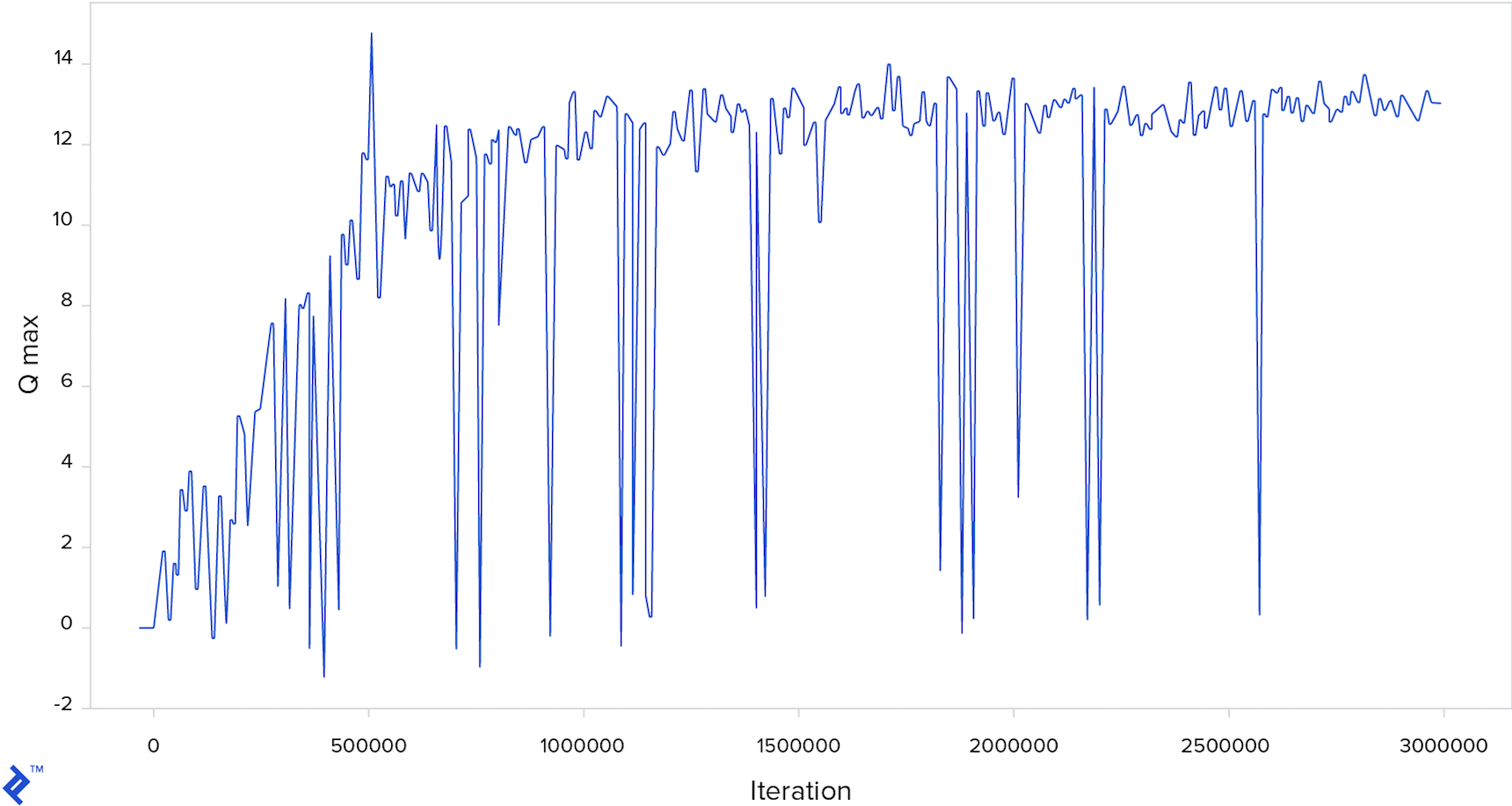
The chart below depicts the evolution of the maximum Q-value throughout the training iterations, with every 10,000th iteration displayed. Downward spikes indicate instances where the neural network predicts a low future reward for a particular frame, suggesting an imminent crash.

The complete source code and a pretrained model are available here.

Deep Reinforcement Learning: 2D, 3D, and Even Real Life

This PyTorch reinforcement learning tutorial demonstrated how a computer, starting with no prior knowledge of Flappy Bird, can learn to play the game through a trial-and-error approach, mimicking the learning process of a human player.

Remarkably, the entire algorithm can be implemented in a concise manner using the PyTorch framework. It’s worth noting that the techniques presented in this blog post are based on a relatively early paper in the field of deep reinforcement learning. Since then, numerous advancements have been made, leading to faster convergence and improved performance.

Deep reinforcement learning has transcended the realm of 2D games and found applications in training agents to play 3D games and even control real-world robotic systems.

Companies at the forefront of AI research, such as DeepMind, Maluuba, and Vicarious, are heavily invested in advancing deep reinforcement learning. This technology played a pivotal role in the development of AlphaGo, the AI system that famously defeated Lee Sedol, one of the world’s top Go players. At the time, it was widely believed that it would take at least a decade for machines to reach such a level of proficiency in Go.

The surge of interest and investment in deep reinforcement learning, and artificial intelligence in general, has sparked discussions about the potential emergence of artificial general intelligence (AGI) - human-level or even superhuman intelligence that can be expressed algorithmically and simulated on computers. However, AGI is a topic for another time.

References:

• Demystifying Deep Reinforcement Learning
• Deep Reinforcement Learning for Flappy Bird
• “Convolutional neural network” at Wikipedia
• “Reinforcement learning” at Wikipedia
• “Markov decision process” at Wikipedia
• University College London course on RL