This is Part III of our three-part series on video game physics. For the rest of this series, see:

Part I: An Introduction to Rigid Body Dynamics Part II: Collision Detection for Solid Objects

Part I of this series showed us how to simulate the movement of rigid bodies when they are not affected by any forces. Part II demonstrated how to make bodies aware of each other through tests that detect collisions and proximity. However, we still need to understand how to make objects genuinely interact with one another. For instance, although we can detect collisions and get helpful details about them, we haven’t figured out what to do with this information.

To put it differently, we have only addressed unconstrained simulations. The final stage in simulating realistic, solid objects is to implement constraints, which set limits on how rigid bodies can move. Examples of constraints include joints (like ball joints and hinge joints) and non-penetration constraints. This last type is used to resolve collisions, ensuring bodies don’t pass through each other and instead bounce off realistically.

This article will explore equality and inequality constraints in video game physics. We’ll first look at them through a force-based lens, where we figure out corrective forces, and then through an impulse-based lens, where we determine corrective velocities. Finally, we’ll cover some smart ways to streamline the process and speed up calculations.

Get ready for some serious math in this installment, more so than in Part I or Part II. If you need a calculus refresher, Khan Academy has you covered](https://www.khanacademy.org/math/differential-calculus). For a review of linear algebra basics, refer to the [appendix in Part I, and for the more complex linear algebra, such as matrix multiplication, Khan Academy again delivers. Wikipedia also offers comprehensive articles on calculus and linear algebra.

What are Constraints?

Constraints are essentially regulations that must be followed throughout the simulation. Some examples are “these two points on this pair of rigid bodies must always touch” or “the space between these two particles should never exceed 2”. In simple terms, a constraint takes away degrees of freedom from a rigid body. Every step of the simulation involves calculating corrective forces or impulses. These forces, when applied to the bodies, either pull them together or push them apart. This ensures their movement stays within the boundaries set by the constraints.

In a practical sense, a constraint is defined by a behavior function or constraint function C. This function takes the state of two bodies (e.g., their positions and orientations) and produces a single number. The constraint is considered satisfied when the function’s output falls within an acceptable range. Therefore, every step of the simulation involves applying forces or impulses to the rigid bodies to try and maintain the value of C within this permitted range.

An Example: Equality Constraints

A frequently encountered type of constraint is the equality constraint. In an equality constraint, the only valid value for C is zero. As such, we want to keep C as close to zero as possible with every step of the simulation. Put another way, we want to minimize C. Equality constraints are employed when the position of a particle or point must always precisely match a predefined condition. A good example is a ball joint, where two rigid bodies are permanently linked at the joint’s location.

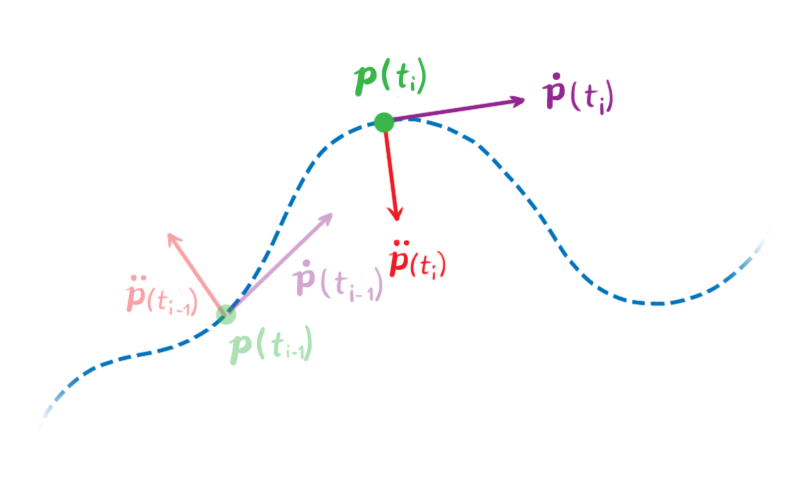
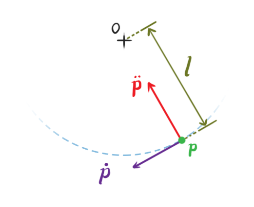
Let’s illustrate with a basic example. Consider a particle in a two-dimensional space. Its position, denoted by p(t) = (px(t), py(t)), is a function of time, providing the particle’s coordinates at a specific time t. We’ll use dot notation to represent time derivatives. This means ṗ is the first time derivative of p concerning time, which represents the particle’s velocity v(t), while p̈ is its second time derivative, or its acceleration.

Let’s establish a constraint. Let C represent the following behavior function:

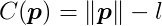
This function uses the particle’s position as input and outputs its distance from the origin minus l. The output will be zero whenever the distance between the particle and the origin is l. This means the constraint’s effect is to keep the particle a constant distance l from the origin, resembling a pendulum fixed at the origin. The values of p that satisfy C(p) = 0 are referred to as the legal positions of the particle.

In this scenario, C depends only on two variables and outputs a single number. This makes it easy to plot and analyze some of its characteristics. If we fix the constraint distance at 2 (l = 2), the graph of C looks like this:

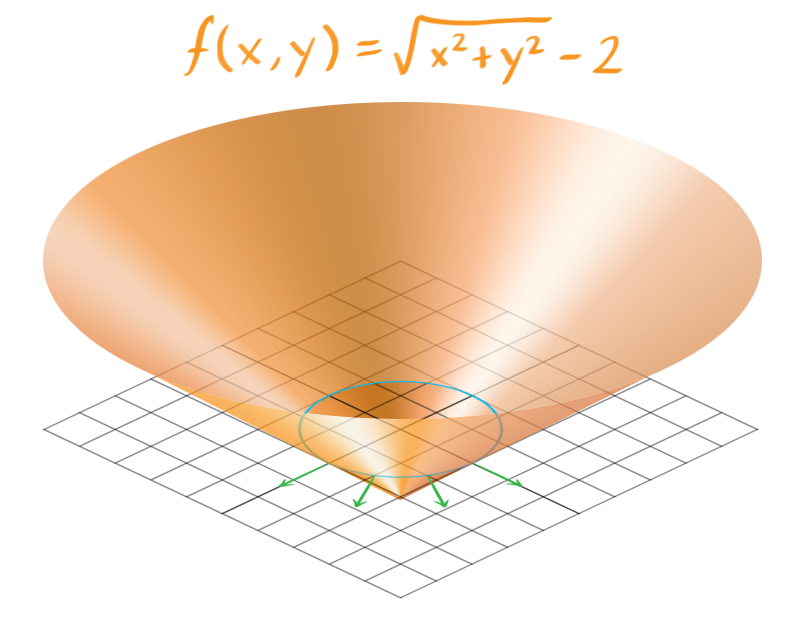
It resembles an upside-down cone. The blue ring marks the points where C = 0, which are the roots of C. This set of points is called the constraint hypersurface, encompassing all the permissible positions for our particle. The constraint hypersurface is an s-dimensional surface, with s being the number of variables in C.

The green arrows represent the gradients of C, calculated around the hypersurface, and point toward the illegal positions of our particle, where C ≠ 0. If the particle moves along these lines, either positively (away from the origin) or negatively (toward the origin), it will break the constraint. This means the forces we produce to push the particle toward legal positions will act parallel to these lines.

While this simplified example has only two variables, most constraint functions have more, making them harder to visualize. But the underlying principle remains the same. Each step requires generating constraint forces that are parallel to the gradient of C at the hypersurface.

Computing Constraint Forces

Ideally, we would just set p in a way that always keeps C exactly at zero. However, in reality, this leads to unrealistic behavior, with our particle erratically jumping and vibrating around the hypersurface. To maintain C as close to zero as possible while ensuring realistic behavior, an intuitive approach is to use force-based dynamics. This involves calculating the necessary force to apply to the particle so that it adheres to the constraints without defying Newton’s laws of motion.

To calculate the constraint force, we need to understand the particle’s permissible accelerations and velocities. To do this, we must find the derivatives of C concerning time.

We want to guarantee that the value of C stays at zero, constant throughout the simulation. This means the first time derivative, Ċ, must also be zero.

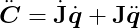
Similarly, for Ċ to remain at zero, the second derivative, C̈, must also be zero.

We don’t need to constrain further derivatives of C because our constraint forces will be applied at the second derivative.

Let’s figure out these derivatives. Our current C definition uses a square root, which makes differentiation a bit tricky. However, we can rephrase C using squared distances:

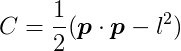
This doesn’t change the fact that C will be zero when the distance between the particle and the origin is l. From this, we can obtain the first derivative of C with respect to t:

For a given legal position of p, all velocities ṗ that satisfy Ċ(p) = 0 are considered legal velocities. In this example, these should be only the velocities tangential to the hypersurface in the previous image.

The second derivative of C concerning t is:

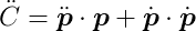
Put differently, given a legal position and velocity, all accelerations p̈ that satisfy C̈(p) = 0 are legal accelerations. In our example, these should only be accelerations directed toward or away from the origin.

We can use Newton’s Second Law of motion to express acceleration in terms of force. Let’s assume two forces act on the particle: a combination of all external forces _f_ext (like gravity, wind, or user-applied forces) and the constraint force _f_C (which we’re trying to determine). Assuming the particle has mass m, its acceleration can be expressed as:

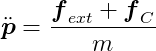
Substituting this into C̈ = 0, we get:

This can be rearranged to:

We have one equation and two unknowns (the two coordinates of _f_C), making it unsolvable as is. We need another condition.

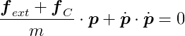
Intuitively, we know that the constraint force must act against the direction we want to prevent the particle from moving in. In this example, constraint forces will always point perpendicular to the circle of radius l because the particle can’t move outside this circle. These perpendicular forces will push the particle back onto the circular path if it tries to deviate, making the velocity component in those directions zero. Therefore, constraint forces will always be perpendicular to the particle’s velocity.

As a result:

The equation for our constraint’s first derivative states that p · ṗ = 0. Since _f_C · ṗ = 0, we know that both _f_C and p are orthogonal to ṗ, meaning _f_C and p are parallel. We can then express one as a multiple of the other:

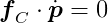
Almost there! The scalar λ represents the magnitude of the constraint force required to bring the system to a valid state. The further our system strays from valid states, the larger λ becomes to push it back. Currently, λ is our only unknown. Substituting the above into our previous equation gives:

We can now directly calculate λ and obtain _f_C by multiplying it by p. Then, we simply apply _f_C to the particle and let the simulation described in Part I handle the rest!

λ is also known as a Lagrange multiplier. For any constraint, the calculation involves determining the direction of the force vector and its magnitude, λ.

When to Apply Constraint Forces

This example shows that computing constraint forces requires knowing all other forces (_f_ext). Of course, we must apply constraint forces before simulating the resulting motion. Therefore, a generalized sequence for each simulation step looks like this:

1. Calculate all external forces _f_ext.
2. Calculate the constraint forces _f_C.
3. Apply all forces and simulate the motion, as outlined in Part I.

Systems of Constraints

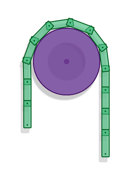
That was a relatively simple example of a very basic constraint involving a single entity. In reality, we want to be able to have numerous constraints and many objects in our simulation. We can’t handle constraints in isolation because the forces applied by one constraint might affect the forces another constraint applies. This is clearly visible in a chain of rigid bodies connected by revolute joints. Consequently, constraints must be solved as a whole system of equations.

Setting Up

We’ll now work with vectors and matrices that represent the state of all entities in our simulation. We’ll use these to develop our global equations, similar to what we did for the single-particle example. Let’s develop these equations for rigid bodies in two dimensions.

State Vector

Suppose we’re simulating n rigid bodies. Let q be a state vector containing the positions and angles of all rigid bodies:

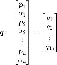
where _p_i is a two-dimensional vector representing the position of the i-th rigid body, and α__i is its angle, a scalar value. Therefore, q has 3n elements.

Dynamics: Newton’s Second Law

Let M represent the following 3n by 3n diagonal matrix:

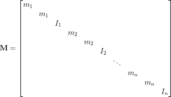
where m__i is the mass of the i-th rigid body, and I__i is its moment of inertia.

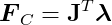
Let F represent a global force vector containing the forces and torques acting on each body. It’s the sum of external and constraint forces:

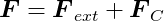
and:

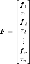
F also has 3n elements, as each _f_i is a two-dimensional vector.

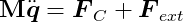
We can now write Newton’s Second Law of motion for the entire set of bodies with a single expression:

Constraints

Finally, let’s set up our behavior functions. Suppose there are m constraints, each like a link in our chain of rigid bodies. We’ll combine all our behavior functions into a single function C(q):

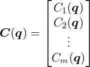
C(q) takes the 3n-dimensional vector q as input and outputs an m-dimensional vector. We aim to keep this output as close to the zero vector as possible, similar to our previous approach.

We won’t delve into defining each behavior function here, as it’s not necessary for our purposes, but there are excellent online tutorials on revolute joint constraints.

Derivatives of C Over Time

As before, we want the first and second time derivatives of C to be zero vectors. Let’s formulate these equations.

The derivative of C concerning time can be expressed as:

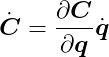
Note the use of the chain rule. We can further develop this equation by defining J as:

This is known as the Jacobian Matrix or the Jacobian of C. The Jacobian generalizes the gradient, which itself generalizes the concept of slope. It’s also worth noting that each row represents the gradient of each behavior function. The Jacobian tells us how each behavior function responds to changes concerning each state variable.

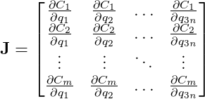
In our chain example, the Jacobian will be a sparse matrix. This is because each constraint only involves the two rigid bodies connected by it. The state of other bodies doesn’t directly affect that specific link.

We can now express the time derivative of C as:

Elegant, isn’t it?

The second derivative of C is:

where:

Substituting our expression of Newton’s Second Law gives:

Computing the Constraint Force Vector

Since we want the second derivative of C to be zero, let’s set it to zero and rearrange:

This equation resembles the one we derived earlier for a single constraint:

Once more, we have more unknowns than equations. Again, we can leverage the fact that constraint forces are orthogonal to velocities to find a solution:

We also want the first derivative of C to be zero. From Ċ = 0, we have:

Therefore, we can express the constraint force vector _F_C as a multiple of J:

The vector λ has m scalar components. In this matrix-vector multiplication, each component λ__i multiplies a row of J (the gradient of the i-th constraint function) and sums them up. That is:

So, _F_C is a linear combination of the rows of J, which are the gradients of our constraint functions. Even though visualizing the hypersurface is challenging in this complex system, as we did for the single-particle example, it behaves in the same way. The gradients are orthogonal to the constraints’ hypersurfaces and represent directions the system cannot move in. This means we have a linear combination of vectors pointing in the forbidden directions. Consequently, the constraint forces are confined to these directions and will push the bodies towards states allowed by the constraints.

The only remaining task is to solve for the λ vector, which determines the magnitudes of our constraint forces. Let’s return to our main equation and substitute the last expression:

This is a system of linear equations where only λ is unknown. Fortunately, plenty of well-established methods can efficiently solve such linear systems. Once we solve for λ, we can calculate _F_C, apply the results to the rigid bodies, and simulate the resulting motion, as shown in Part I.

For a more detailed derivation of these equations, check out Andrew Witkin’s Constrained Dynamics, which is part of the Physically Based Modeling: Principles and Practice course at Carnegie Mellon University.

Inequality Constraints

We’ve assumed so far that our behavior functions must always equal zero for constraints to be satisfied. However, some constraint types require more flexibility, where corrective forces aren’t applied for a broader range of C values, not just zero. One example is the non-penetration constraint, crucial in rigid body simulations. It handles collision resolution, preventing unrealistic interpenetration of bodies and giving them a natural solid behavior.

As discussed in Part II, after the GJK algorithm detects a collision, we know the contact points on both bodies and the surface normal at the contact point. Remember that GJK is both a collision and a proximity test. Two bodies might be considered “colliding” even without touching if the distance between them is very small. In this case, the contact points are the points on the two bodies closest to each other.

The non-penetration constraint aims to keep bodies separate by applying corrective forces that push them apart, but only when the bodies are colliding.

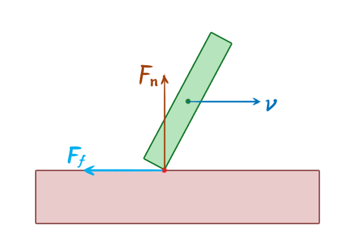
Consider two colliding 2D bodies, A and B. At the moment of contact, A has position _p_A and angle α__A, while B has position _p_B and angle α__B. Let _r_A be a vector from the center of A to the contact point on A, and define _r_B similarly. Let n be the contact normal pointing from A to B.

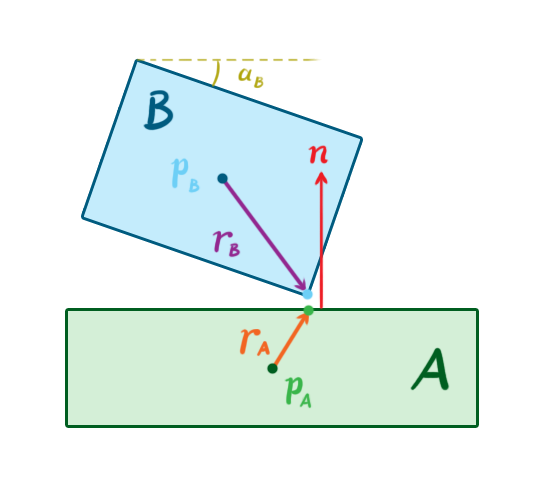
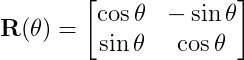
Let’s use a standard 2D rotation matrix R(θ) that rotates vectors by an angle θ:

We can rotate the vectors _r_A and _r_B by the angles α__A and α__B, respectively, using this matrix. This allows us to define a behavior function, C, as:

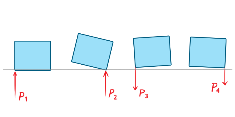
This behavior function might look intimidating, but its action is straightforward. It takes a vector between the contact point on A and the contact point on B, projects it onto the normal vector n, and outputs the projected vector’s length. In other words, it calculates the penetration depth along the normal. If C is greater than or equal to zero, no force should be applied because the bodies are not penetrating. Therefore, we need to enforce the inequality C ≥ 0.

Analyzing the equations reveals that we only need to restrict the value of λ for each constraint. In our previous equality constraint examples, λ could be any value, meaning the constraint forces could act in either a positive or negative direction along the behavior gradients. However, in an inequality constraint like the non-penetration constraint, λ must be greater than or equal to zero. This signifies that constraint forces can only push the colliding bodies away from each other.

This change transforms our linear system of equations into something different (and more complex) called a Mixed Linear Complementarity Problem, or MLCP. There are efficient algorithms for directly solving this problem, such as Lemke’s Algorithm. However, we’ll skip the details here and discuss a popular alternative approach to constraints in game physics.

Impulse-Based Dynamics

So far, we’ve explored the force-based method for enforcing constraints. We calculate constraint forces, apply them to the bodies along with external forces, and integrate them using the methods from Part I to simulate the resulting motions. However, another popular technique among game physics engines takes an impulse-based approach. This method works with the velocity of the bodies instead of their force or acceleration. In this approach, the constraint solver calculates and applies a direct change to the linear and angular velocities of the bodies, rather than relying on calculating and applying corrective forces and then using integration to modify the velocities.

With impulse-based dynamics, the goal is to determine the impulses that result in velocities that satisfy the constraints. This is somewhat similar to the force-based goal of finding the forces that produce accelerations satisfying the constraints. However, we’re working at a lower order of magnitude, and as a result, the math is less complicated.

Brian Mirtich popularized the impulse-based approach in his PhD thesis from 1996, which remains a key reference on the subject. Jan Bender et. al. have also published a series of significant papers on this topic.

The typical sequence of a simulation step using impulse-based dynamics differs slightly from the force-based approach:

1. Calculate all external forces.
2. Apply the forces and determine the resulting velocities, as explained in Part I.
3. Calculate the constraint velocities based on the behavior functions.
4. Apply the constraint velocities and simulate the resulting motion.

Perhaps the most significant advantage of impulse-based dynamics over force-based and other methods is its relative algorithmic simplicity. It’s also more intuitive to grasp. In most cases, it’s computationally more efficient, making it attractive for games where real-time performance is paramount. However, there are drawbacks, including challenges in realistically handling stable contacts (like a stack of boxes at rest) and increased complexity when modeling contact friction. Nevertheless, we can address these issues in several ways, as we’ll see later.

In physics, an impulse is the integral of a force over time. That is:

This is equivalent to the change in momentum during that time.

If a constant force F is applied for a time h, the impulse is simply:

When two rigid objects collide, their contact lasts for a very short time, during which they deform and exert equal and opposite forces on each other. After this brief interaction, their velocities, and consequently their momentums, may change significantly. If the objects were perfectly rigid, their contact time would be infinitesimally small, and their velocities would change instantly upon collision. Perfectly rigid bodies don’t exist in the real world, but we can use this simplification to realistically simulate the behavior of very rigid objects.

Sequential Impulses

Our objective is to find the impulses that satisfy the constraints for the current simulation step. One technique for achieving this is called sequential impulses, popularized by Erin Catto, the creator of the Box2D physics engine. This iterative algorithm aims to zero in on the constraint velocity by applying impulses to the rigid bodies with each iteration, repeating until the resulting velocity error is negligible—in other words, until Ċ is very close to zero.

Unlike our previous approach, sequential impulses don’t involve creating one large system of equations and inequalities. Instead, we model and solve each constraint individually, much like our first example with a single particle. The algorithm can be summarized in three steps:

1. Integrate applied forces using semi-implicit Euler, as shown in Part I, to obtain tentative velocities. These velocities might violate the constraints and need correction before application.

2. Apply impulses sequentially to all constraints to correct velocity errors. Repeat this process over several iterations until the impulses become very small or a maximum iteration count is reached.

3. Use the new velocities to simulate motion and update positions, again employing semi-implicit Euler.

Note that these steps correspond to steps 2 through 4 in the general impulse-based time step sequence described earlier.

Computing the Velocities

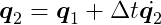
Let’s examine the equations. Let _q̇_1 = q̇(t__i-1) and _q̇_2 = q̇(t__i). In other words, _q̇_1 and _q̇_2 are the velocities in the previous and current time steps, respectively (we’re trying to determine the latter). Using semi-implicit Euler integration, the tentative, unconstrained velocity for the current step (indicated by an asterisk) is:

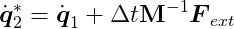
This velocity might violate the constraints, in which case we need to correct it with an impulse.

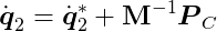
Let _P_C represent the constraint impulse. Dividing it by mass gives us the change in velocity, which we then apply to the tentative velocity to get the desired velocity that satisfies the constraints:

So how do we determine _P_C? Recognizing that the impulse will act in the same direction as an instantaneous force producing it, we can again use the fact that constraint forces must be parallel to the gradient of the behavior function, just as we did with force-based constraints. This allows us to write:

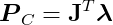
where λ is once again a vector of magnitudes.

The impulse-based approach bypasses Newton’s Second Law, offering a shortcut. By skipping the calculation of forces and their resulting accelerations, it can lead to noticeable, instantaneous velocity changes that might introduce undesirable jitter into a simulation. To mitigate this, it’s common to introduce a bias factor to the velocity constraints, softening the effect:

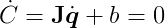
Notice that J_q̇_2 + b = 0, as _q̇_2 must be a valid velocity. Substituting and rearranging the valid velocity equation yields:

After solving this equation for λ, we can compute the constraint impulse using PC = JTλ and finally update the velocity.

We have to solve each constraint individually, apply the impulses, update the bodies’ velocities, and repeat this process multiple times until we achieve convergence or hit the maximum iteration count. This means we accumulate the impulses as we iterate. To complete the time step, we simply update the positions using the final velocities:

Inequality Constraints

For inequality constraints, we must bound the impulses and keep them within the permitted values during accumulation. This ensures that the constraints don’t apply impulses with inappropriate directions or strengths. This bounding process isn’t as simple as applying a min/max function because we only want to bound the final accumulated impulse, not the intermediate impulses generated during accumulation. For details, check out Erin Catto’s GDC 2009’s presentation.

Warm Starting

One effective technique for enhancing the algorithm’s accuracy is called warm starting. The algorithm starts with an initial guess for λ and works from there. Considering the significant temporal and spatial coherence in physics simulations, it’s natural to use the λ from the previous step as a starting point, which is precisely what warm starting does. Since bodies often don’t move much between steps, the impulses calculated in the previous step are likely to be very similar in the current step. Starting our algorithm from this point helps it converge to a more accurate solution faster, improving the simulation’s stability, particularly for constraints like joints and persistent contact between bodies.

Projected Gauss-Seidel

Another technique for solving impulse-based constraints stems from the fact that it can also be modeled as an MLCP. Projected Gauss-Seidel (PGS) is an iterative algorithm for solving MLCPs that works well for impulse-based dynamics. It effectively solves a linear system Ax = b with bounds on x. PGS extends the Gauss-Seidel method by bounding the value of x in each iteration to keep it within the desired range.

Since we’re working with velocity, we can eliminate acceleration by approximating it as the ratio of velocity change to the time step’s delta time. Let _q̇_1 = q̇(t__i-1) and _q̇_2 = q̇(t__i), then:

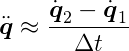
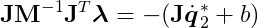
where, again, _q̇_1 represents the velocity calculated in the previous step, and _q̇_2 is the velocity we want for the current step. From Newton’s Second Law, we have:

Substituting our approximation and FC = JTλ gives us:

Since Ċ = 0, we know that J_q̇_2 = 0 because _q̇_2 will be a legal velocity after solving this. Rearranging and multiplying both sides by J yields:

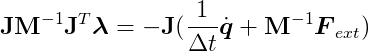
This MLCP differs slightly from the force-based approach because it uses an approximate acceleration. Once we solve it using PGS, we’ll have λ, and we can then calculate _q̇_2 using the previous equation:

We can easily obtain the updated positions and orientations from the semi-implicit Euler scheme:

Interestingly, closer inspection reveals that PGS is equivalent to sequential impulses! We’re essentially doing the same thing. We can again employ warm starting, using the λ computed in the previous step as our starting point. The difference is that the sequential impulses formulation is more intuitive, while the PGS formulation is more general, allowing for more flexible code. For example, we could experiment with different tools for solving the MLCP.

For a deeper dive into using PGS in an impulse-based simulation, refer to Erin Catto’s 2005 GDC presentation and paper.

Simulating Friction Using Impulses

The Coulomb friction model is straightforward and effective. It outlines two scenarios when two solid surfaces are in contact:

• Static friction: This is the resistance to tangential motion when the surfaces aren’t moving relative to each other because the force isn’t strong enough to overcome friction. The friction force acts in the opposite direction of the net tangent force and has the same magnitude.
• Kinetic friction: This is the resistance to tangential motion when the surfaces are sliding against each other. The friction force opposes the direction of motion and has a smaller magnitude than the net tangent force.

The friction force is proportional to the normal force, which is the net force component acting perpendicular to the contact surface. In simpler terms, the force of friction is proportional to the force pushing the two objects together. It can be expressed as:

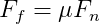
where F__f is the friction force, F__n is the normal force, and μ is the coefficient of friction (which can differ for static and kinetic friction).

To simulate friction using a constraint model, we must formulate a velocity constraint directly:

Here, _v_p represents the relative velocity vector at the contact point p, and t is a unit vector tangent to the surfaces. The goal is to reduce the tangential velocity to zero.

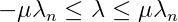
According to the friction equation, we must limit the friction impulse to the normal impulse multiplied by the coefficient of friction. This means keeping our λ between -μ _λ_n and μ _λ_n, where _λ_n is the magnitude of the normal impulse.

Therefore, friction is another instance of an inequality constraint.

Things become slightly more complex in three dimensions. In his 2005 GDC presentation, Erin Catto presents an approach that uses two tangent vectors and two constraints. However, limiting the friction impulse to a multiple of the normal impulse in this case couples the two constraints, making them challenging to solve. To work around this, he limits the friction impulse by a constant value proportional to the body’s mass and the acceleration due to gravity.

Optimizations

We’ve covered several methods for determining the forces or impulses to apply to our rigid bodies to enforce constraints. Each of these methods involves a fair amount of computation. Let’s explore some clever optimization strategies to reduce unnecessary work.

Islands

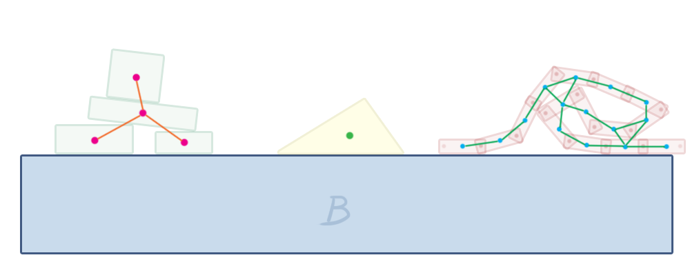
In a constrained physics simulation, some objects influence the motion of others, while others don’t.

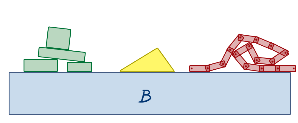
In the image above, box B is a static object, representing the floor. The objects on the left are stacked, making contact with each other. If any of these objects move, the others might move as well due to the contact constraints between them. Any force or impulse applied to these bodies may propagate through the stack. However, the triangle in the middle rests independently on the stationary box B. Forces applied to the stacked objects on the left will never affect the triangle because there’s no connection between them. The same applies to the chain of boxes on the right. They are all connected by revolute joints, so the movement of one box can create a reaction along the constraints, influencing the motion of other boxes in the chain. But they will never affect the triangle or the stacked objects on the left unless a new constraint is created between them, such as a contact/non-penetration constraint arising from a collision due to their movement.

This observation allows us to group objects into islands, which are self-contained groups of bodies that can influence each other’s motion through constraint forces/impulses but won’t affect objects in other islands.

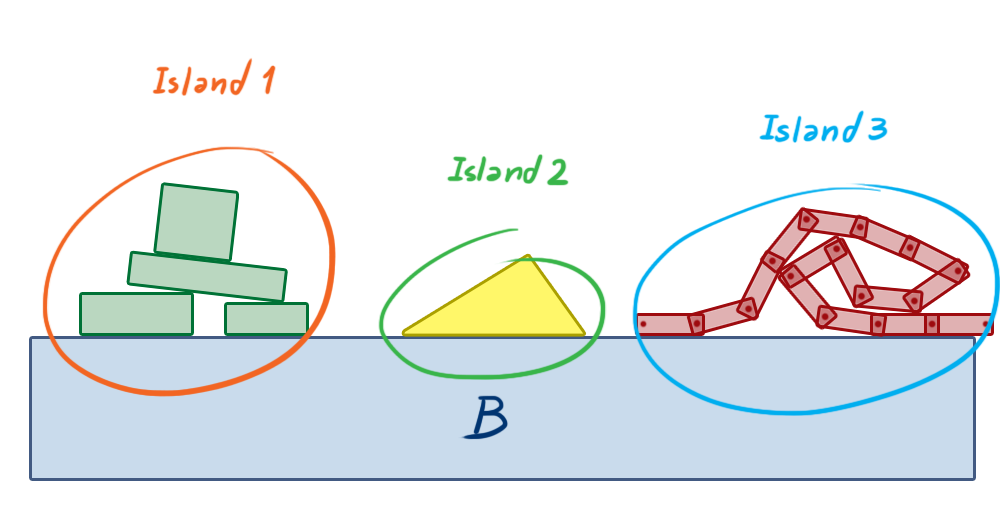
This separation allows us to solve smaller constraint groups, creating smaller systems instead of one large system for the entire physics world. This eliminates a potentially massive amount of unnecessary computation.

If we view the world as a graph where bodies are nodes and constraints are edges, we can construct the islands using a depth-first search on this graph. In graph theory, our islands are called connected components.

Box2D does this in its b2World::Solve method, which is responsible for solving all constraints in each step. It constructs the islands and calls b2Island::Solve on each, which then solves the constraints within that island using sequential impulses.

Sleeping

When a body in the simulation comes to rest, its position naturally remains constant in subsequent steps unless an external force causes it to move again. This presents another optimization opportunity: we can stop simulating an island if the linear and angular velocities of all its bodies remain below a certain threshold for a short period. This condition is called sleeping.

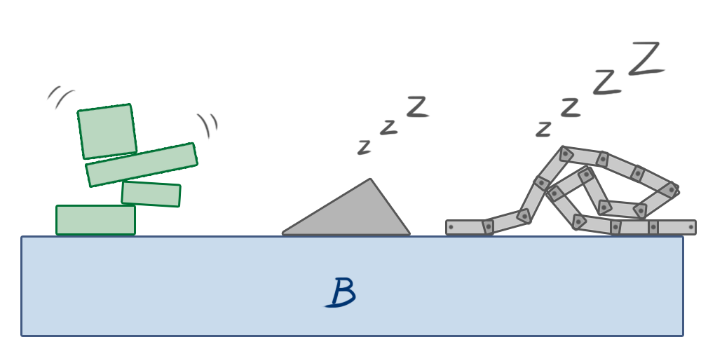
Once an island is asleep, its bodies are excluded from all simulation steps except collision detection. If a body outside the island collides with a body in the sleeping island, the island “wakes up” and rejoins the simulation. Similarly, if an external force or impulse is applied to one of its bodies, the island wakes up.

This simple technique can dramatically improve the performance of simulations with many objects.

Conclusion - Video Game Physics and Constrained Rigid Body Simulation

This concludes our three-part series on video game physics. We’ve explored how to simulate physics in games, focusing on rigid body simulation, a fundamental aspect of physics simulation that can make games more dynamic and enjoyable. We’ve learned how to simulate the motion of rigid bodies, detect and resolve collisions between them, and model other interactions.

Widely used game physics engines like Box2D, Chipmunk Physics, and Bullet Physics employ the techniques we’ve explored. These approaches enable the creation of games with lifelike, dynamic behavior, allowing objects to move, collide, and connect in various ways using different joint types. Interestingly, these methods also have applications beyond gaming, such as in robotics.

However, practical implementation often presents challenges not predicted by theory. Achieving a stable and efficient implementation, especially for constrained dynamics, requires numerous ingenious simplifications. While significant advancements have been made in collision detection, time of impact computation, MLCP resolution, and more, there’s still room for improvement. The Bullet Physics Forum provides a valuable resource for staying informed about the latest developments in game and rigid body physics simulation, particularly the Research and development discussion about Collision Detection and Physics Simulation section where members discuss cutting-edge simulation techniques.