OpenGL is a versatile cross-platform API that grants developers deep access to system hardware across various programming environments.

Why choose OpenGL?

It offers low-level graphics processing for both 2D and 3D, eliminating performance bottlenecks often encountered with interpreted or high-level languages. More significantly, it unlocks hardware-level access to the GPU, a game-changer for graphics-intensive tasks.

While individual GPU cores are slower than CPU cores, the GPU shines in parallel processing. By deploying small programs called “shaders,” we can harness the combined power of hundreds of GPU cores, enabling the simultaneous execution of repetitive tasks that would cripple a CPU.

This article guides you through building a rudimentary Android application that leverages OpenGL for on-screen content rendering. Prerequisites include familiarity with Android development and the syntax of a C-like language. The complete source code for this tutorial is available on GitHub.

OpenGL Tutorial and Android

To showcase OpenGL’s capabilities, we’ll craft a deceptively simple Android application: a Mandelbrot set generator. The Mandelbrot set is rooted in the realm of complex numbers. Given the vastness of complex analysis, our focus will remain on the visual output rather than delving into the underlying mathematics.

Version Support

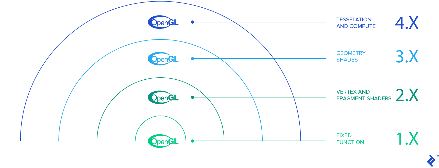
To ensure compatibility, we’ll target devices with OpenGL 2.0 support. Within your manifest file, between the manifest and application declarations, specify OpenGL 2.0 usage:

1

<uses-feature android:glEsVersion="0x00020000" android:required="true" />

While OpenGL 3.0 and 3.1 are gaining traction, targeting these versions might exclude roughly 65% of devices. Opt for these only if the added functionality outweighs compatibility concerns. They can be implemented by setting the version to ‘0x000300000’ and ‘0x000300001’ respectively.

Application Architecture

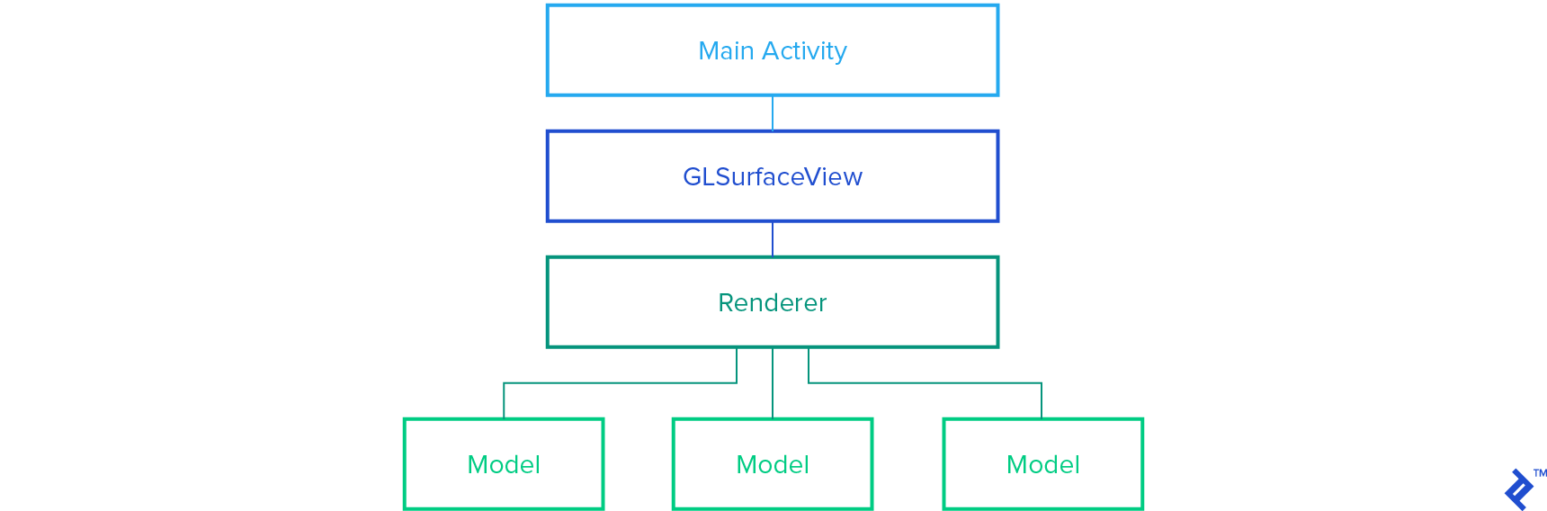
Our OpenGL Android application will typically consist of three primary classes responsible for surface drawing: MainActivity, an extension of GLSurfaceView, and an implementation of a GLSurfaceView.Renderer. From these, we will create various Models to encapsulate drawings.

MainActivity, named FractalGenerator in this example, primarily instantiates the GLSurfaceView and manages global changes. Here’s a boilerplate example:

 1
 2
 3
 4
 5
 6
 7
 8
 9
10
11
12
13
14
15
16
17
18
19
20
21
22
23
24
25
26
27
28

public class FractalGenerator extends Activity {

	private GLSurfaceView mGLView;

	@Override
	public void onCreate(Bundle savedInstanceState) {
		super.onCreate(savedInstanceState);

		//Create and set GLSurfaceView
		mGLView = new FractalSurfaceView(this);
		setContentView(mGLView);
	}

	//[...]

	@Override
	protected void onPause() {
		super.onPause();
		mGLView.onPause();
	}

	@Override
	protected void onResume() {
		super.onResume();
		mGLView.onResume();
	}

}

This class is also suitable for housing other activity-level modifications, such as immersive fullscreen).

Next, we have an extension of GLSurfaceView, serving as our primary view. Within this class, we configure the OpenGL version, set up a Renderer, and handle touch events. The constructor involves setting the OpenGL version using setEGLContextClientVersion(int version) and creating/setting the renderer:

1
2
3
4
5
6
7
8

public FractalSurfaceView(Context context){
	super(context);
	
	setEGLContextClientVersion(2);

	mRenderer = new FractalRenderer();
	setRenderer(mRenderer);
}

Attributes like the render mode can be configured using setRenderMode(int renderMode). Given the computational cost of Mandelbrot set generation, we’ll employ RENDERMODE_WHEN_DIRTY, rendering the scene only during initialization or upon explicit calls to requestRender(). Refer to the GLSurfaceView API for additional configuration options.

Besides the constructor, consider overriding the onTouchEvent(MotionEvent event) method for managing touch-based user input. However, we’ll skip the specifics as they fall outside this lesson’s scope.

Finally, we arrive at the Renderer, where the bulk of lighting and scene manipulation occurs. Before proceeding, let’s briefly touch upon matrices and their role in the graphics realm.

Quick Lesson in Linear Algebra

Matrices are fundamental to OpenGL, offering a concise representation of sequential generalized changes in coordinates. They empower us to perform rotations, scaling, reflections, and even translations with a bit of ingenuity. In essence, matrices facilitate any desired reasonable change, from camera movement to object scaling. By multiplying our matrices by a vector representing coordinates, we can effortlessly generate the transformed coordinate system.

OpenGL provides the Matrix class, offering pre-built methods for common matrix calculations. However, understanding their mechanics is beneficial even for simple transformations.

Let’s address the use of four-dimensional vectors and matrices for coordinate handling. This stems from the need to enable translations. While impossible in 3D space using only three dimensions, adding a fourth dimension unlocks this capability.

Consider this basic scale/translation matrix:

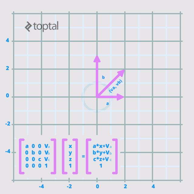
Importantly, OpenGL matrices are column-wise. Therefore, this matrix would be represented as {a, 0, 0, 0, 0, b, 0, 0, 0, 0, c, 0, v_a, v_b, v_c, 1}, differing from the conventional reading order. This ensures consistency with vectors, which are treated as columns during multiplication.

Back to the Code

Equipped with this matrix knowledge, let’s resume designing our Renderer. A common practice involves creating a matrix within this class, formed by multiplying three matrices: Model, View, and Projection, aptly named the MVPMatrix. For an in-depth explanation, refer to here. Given the Mandelbrot set’s nature as a fullscreen 2D model, we’ll forego the concept of a camera and utilize a simpler set of transformations.

Let’s set up the Renderer class. We’ll implement the required methods methods of the Renderer interface: onSurfaceCreated(GL10 gl, EGLConfig config), onSurfaceChanged(GL10 gl, int width, int height), and onDrawFrame(GL10 gl). The complete class will resemble this:

 1
 2
 3
 4
 5
 6
 7
 8
 9
10
11
12
13
14
15
16
17
18
19
20
21
22
23
24
25
26
27
28
29
30
31
32
33
34
35
36
37
38
39
40
41
42
43
44
45
46
47
48
49

public class FractalRenderer implements GLSurfaceView.Renderer {

	//Provide a tag for logging errors
	private static final String TAG = "FractalRenderer";
	
	//Create all models
	private Fractal mFractal;

	//Transformation matrices
	private final float[] mMVPMatrix = new float[16];

	//Any other private variables needed for transformations
	
	@Override
	public void onSurfaceCreated(GL10 unused, EGLConfig config) {
		// Set the background frame color
		GLES20.glClearColor(0.0f, 0.0f, 0.0f, 1.0f);

		//Instantiate all models
		mFractal = new Fractal();
	}

	@Override
	public void onDrawFrame(GL10 unused) {
	//Clear the frame of any color information or depth information
	GLES20.glClear(GLES20.GL_COLOR_BUFFER_BIT | GLES20.GL_DEPTH_BUFFER_BIT);

	//Create a basic scale/translate matrix
		float[] mMVPMatrix = new float[]{
				-1.0f/mZoom,  0.0f,                0.0f,    0.0f,
				0.0f,        1.0f/(mZoom*mRatio), 0.0f,    0.0f,
				0.0f,        0.0f,                1.0f,    0.0f,
				-mX,         -mY,                0.0f,    1.0f};

		//Pass the draw command down the line to all models, giving access to the transformation matrix
		mFractal.draw(mMVPMatrix);
	}

	@Override
	public void onSurfaceChanged(GL10 unused, int width, int height) {
		//Create the viewport as being fullscreen
		GLES20.glViewport(0, 0, width, height);
	
		//Change any projection matrices to reflect changes in screen orientation
	}

	//Other public access methods for transformations

}

Two utility methods, checkGLError and loadShaders, are included for debugging and shader management.

Notice how we delegate tasks down the chain of command, encapsulating different program aspects. We’ve finally reached the point of defining the program’s core functionality. This involves creating a “Model” class to hold the display information for each scene object. In complex 3D scenes, this could represent an animal or object; our simpler 2D example utilizes a fractal.

Model classes are self-contained, requiring no mandatory superclasses. They simply need a constructor and a “draw” method with relevant parameters.

However, some boilerplate variables are essential. Let’s examine the constructor used in the Fractal class:

 1
 2
 3
 4
 5
 6
 7
 8
 9
10
11
12
13
14
15
16
17
18
19
20
21
22
23
24
25
26
27
28
29
30
31
32
33
34
35
36
37

public Fractal() {
	// initialize vertex byte buffer for shape coordinates
	ByteBuffer bb = ByteBuffer.allocateDirect(
			// (# of coordinate values * 4 bytes per float)
			squareCoords.length * 4);
	bb.order(ByteOrder.nativeOrder());
	vertexBuffer = bb.asFloatBuffer();
	vertexBuffer.put(squareCoords);
	vertexBuffer.position(0);

	// initialize byte buffer for the draw list
	ByteBuffer dlb = ByteBuffer.allocateDirect(
			// (# of coordinate values * 2 bytes per short)
			drawOrder.length * 2);
	dlb.order(ByteOrder.nativeOrder());
	drawListBuffer = dlb.asShortBuffer();
	drawListBuffer.put(drawOrder);
	drawListBuffer.position(0);

	// Prepare shaders
	int vertexShader = FractalRenderer.loadShader(
			GLES20.GL_VERTEX_SHADER,
			vertexShaderCode);
	int fragmentShader = FractalRenderer.loadShader(
			GLES20.GL_FRAGMENT_SHADER,
			fragmentShaderCode);
			
	// create empty OpenGL Program
	mProgram = GLES20.glCreateProgram();             
	
	// add the vertex shader to program
	GLES20.glAttachShader(mProgram, vertexShader);   
	// add the fragment shader to program
	GLES20.glAttachShader(mProgram, fragmentShader);
	// create OpenGL program executables
	GLES20.glLinkProgram(mProgram);                  
}

While seemingly complex, this part requires minimal modification beyond changing the model name and adjusting class variables accordingly.

Let’s break down some variable declarations:

1
2
3
4
5
6
7

static float squareCoords[] = {
		-1.0f,  1.0f, 0.0f,   // top left
		-1.0f, -1.0f, 0.0f,   // bottom left
		1.0f, -1.0f, 0.0f,   // bottom right
		1.0f,  1.0f, 0.0f }; // top right

private final short drawOrder[] = { 0, 1, 2, 0, 2, 3 }; // order to draw vertices

squareCoords defines the square’s coordinates. On-screen coordinates are represented on a grid where (-1,-1) corresponds to the bottom left and (1,1) to the top right.

drawOrder dictates the order of coordinates to form triangles representing the square. OpenGL relies on triangles for efficient surface representation. To create a square, we divide it diagonally (from 0 to 2 in this case), resulting in two triangles.

To utilize these within the program, convert them to a raw byte buffer. This enables direct interaction between the array contents and the OpenGL interface. Java stores arrays as objects with additional information incompatible with OpenGL’s pointer-based C arrays. ByteBuffers solve this by providing access to the array’s raw memory.

With vertex and draw order data in place, let’s create our shaders.

Shaders

Two shaders are crucial for each model: a Vertex Shader and a Fragment (Pixel) Shader. Shaders are written in GL Shading Language (GLSL), a C-based language augmented with built in functions, variable modifiers, primitives, and default input/output. In Android, these are passed as final Strings through loadShader(int type, String shaderCode), one of the Renderer’s resource methods. Let’s explore the different qualifier types:

• const: Declares final variables as constants for easy access and efficient storage. For example, frequently used values like π can be declared as constants. The compiler might automatically assign constants based on the implementation.
• uniform: Uniform variables remain constant for a single rendering pass, acting like static arguments passed to shaders.
• varying: When declared as varying and set in a vertex shader, these variables are linearly interpolated in the fragment shader. This is valuable for creating gradients and is implicit for depth changes.
• attribute: Non-static arguments to a shader, representing vertex-specific inputs. They only appear in Vertex Shaders.

Additionally, two new primitive types are introduced:

• vec2, vec3, vec4: Floating-point vectors of the specified dimension.
• mat2, mat3, mat4: Floating-point matrices of the specified dimension.

Vectors are accessible through their x, y, z, and w components (or r, g, b, and a). They can also generate vectors of varying sizes using multiple indices: for vec3 a, a.xxyz returns a vec4 with corresponding values from a.

Matrices and vectors can be indexed like arrays, with matrices returning a single-component vector. Thus, for mat2 matrix, matrix[0].a is valid and returns matrix[0][0]. Importantly, treat them as primitives, not objects. Consider the following:

1
2
3

vec2 a = vec2(1.0,1.0);
vec2 b = a;
b.x=2.0;

The result is a=vec2(1.0,1.0) and b=vec2(2.0,1.0). This differs from object behavior, where the second line would assign b a pointer to a.

In our Mandelbrot Set, the Fragment Shader handles most of the generation logic. Vertex Shaders typically operate on vertices and per-vertex attributes like color and depth changes. Let’s analyze the minimalistic vertex shader for our fractal:

1
2
3
4
5

private final String vertexShaderCode =
		"attribute vec4 vPosition;" +
		"void main() {" +
		"  gl_Position = vPosition;" +
		"}";

Here, gl_Position is an OpenGL output variable storing vertex coordinates. We pass a position for each vertex and assign it to gl_Position. In most cases, we would multiply vPosition by an MVPMatrix to transform vertices. However, our fractal remains fullscreen, so transformations occur within a local coordinate system.

The Fragment Shader is where the magic happens. We’ll set fragmentShaderCode to the following:

 1
 2
 3
 4
 5
 6
 7
 8
 9
10
11
12
13
14
15
16
17
18
19
20
21
22
23
24
25
26
27
28
29
30
31

precision highp float;
uniform mat4 uMVPMatrix;

void main() {
	//Scale point by input transformation matrix
	vec2 p = (uMVPMatrix * vec4(gl_PointCoord,0,1)).xy;
	vec2 c = p;

	//Set default color to HSV value for black
	vec3 color=vec3(0.0,0.0,0.0);

	//Max number of iterations will arbitrarily be defined as 100. Finer detail with more computation will be found for larger values.
	for(int i=0;i<100;i++){
		//Perform complex number arithmetic
		p= vec2(p.x*p.x-p.y*p.y,2.0*p.x*p.y)+c;
		
		if (dot(p,p)>4.0){
			//The point, c, is not part of the set, so smoothly color it. colorRegulator increases linearly by 1 for every extra step it takes to break free.
			float colorRegulator = float(i-1)-log(((log(dot(p,p)))/log(2.0)))/log(2.0);
			//This is a coloring algorithm I found to be appealing. Written in HSV, many functions will work.
			color = vec3(0.95 + .012*colorRegulator , 1.0, .2+.4*(1.0+sin(.3*colorRegulator)));
			break;
		}
	}
	//Change color from HSV to RGB. Algorithm from https://gist.github.com/patriciogonzalezvivo/114c1653de9e3da6e1e3
	vec4 K = vec4(1.0, 2.0 / 3.0, 1.0 / 3.0, 3.0);
	vec3 m = abs(fract(color.xxx + K.xyz) * 6.0 - K.www);
	gl_FragColor.rgb = color.z * mix(K.xxx, clamp(m - K.xxx, 0.0, 1.0), color.y);

	gl_FragColor.a=1.0;
}

Most of this code handles the mathematical and algorithmic aspects of the Mandelbrot set. Notice the use of built-in functions like fract, abs, mix, sin, and clamp, operating on and returning vectors or scalars. Additionally, dot takes vector arguments and returns a scalar.

With shaders ready, let’s implement the draw function in our model:

 1
 2
 3
 4
 5
 6
 7
 8
 9
10
11
12
13
14
15
16
17
18
19
20
21
22
23
24
25
26
27

public void draw(float[] mvpMatrix) {
	// Add program to OpenGL environment
	GLES20.glUseProgram(mProgram);

	// get handle to vertex shader's vPosition member
	mPositionHandle = GLES20.glGetAttribLocation(mProgram, "vPosition");
	mMVPMatrixHandle = GLES20.glGetUniformLocation(mProgram, "uMVPMatrix");

	//Pass uniform transformation matrix to shader
	GLES20.glUniformMatrix4fv(mMVPMatrixHandle, 1, false, mvpMatrix, 0);

	//Add attribute array of vertices
	GLES20.glEnableVertexAttribArray(mPositionHandle);
	GLES20.glVertexAttribPointer(
			mPositionHandle, COORDS_PER_VERTEX,
			GLES20.GL_FLOAT, false,
			vertexStride, vertexBuffer);

	// Draw the square
	GLES20.glDrawElements(
			GLES20.GL_TRIANGLES, drawOrder.length,
			GLES20.GL_UNSIGNED_SHORT, drawListBuffer);

	// Disable vertex array
	GLES20.glDisableVertexAttribArray(mPositionHandle);
	FractalRenderer.checkGlError("Test");
}

This function passes all arguments, including the uniform transformation matrix and attribute position, to the shaders.

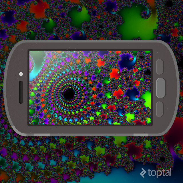
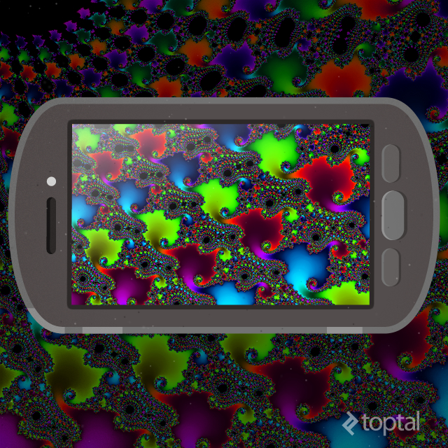
After assembling all components, we can run our application. Assuming proper touch support, we’re greeted with mesmerizing visuals:

Floating Point Accuracy

Zooming in reveals a breakdown in the image:

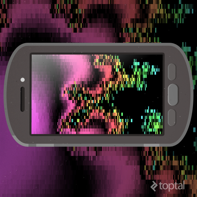
This isn’t a mathematical flaw but a consequence of number representation in OpenGL. While recent versions support double precision, OpenGL 2.0 is limited to floats. Despite using the highest precision floats with precision highp float in our shader, it proves insufficient.

The workaround involves emulate doubles using two floats. While this approach achieves near-native precision, it incurs a significant performance cost. Implementing this for higher accuracy is left as an exercise for the reader.

Conclusion

With a few support classes, OpenGL facilitates real-time rendering of intricate scenes. Combining a GLSurfaceView layout, a custom Renderer, and a model with shaders, we’ve visualized a captivating mathematical structure. May this ignite your passion for developing OpenGL ES applications!