This is the first entry in a three-part series about video game physics. If you’d like to read the rest of the series, you can find the other parts here:

Part II: Collision Detection for Solid Objects Part III: Constrained Rigid Body Simulation

Physics simulation, a fascinating field within computer science, focuses on replicating physical events using the power of computers. These simulations generally employ numerical methods, applying them to established theories to generate results that closely mirror real-world observations. For us, as advanced game developers, this predictive ability is invaluable. It allows us to carefully analyze how something might behave even before we create it in the digital world, saving time and resources.

The applications of physics simulations are incredibly diverse. Early computers, for instance, were already tasked with running physics simulations, such as predicting the trajectory of projectiles for military purposes. Beyond that, it’s a crucial tool in civil and automotive engineering, providing insight into how structures would react to events like earthquakes or car crashes. But it doesn’t stop there. We can simulate incredibly complex phenomena like astrophysics, relativity, and countless other wonders of the natural world.

Simulating physics in video games is commonplace because most games draw inspiration from the world around us. In fact, many games depend entirely on physics simulation for their enjoyment. A physics-based game needs a robust and stable simulation that can handle the demands placed upon it without breaking or slowing down, which is often a difficult task.

In any given game, only specific physical effects truly matter. Rigid body dynamics, which focuses on the movement and interaction of solid, inflexible objects, is by far the most commonly simulated effect in games. This is because most objects we encounter in reality are relatively rigid. Additionally, simulating rigid bodies is less complex (though, as we will see, it’s not exactly a walk in the park). However, some games demand the simulation of more intricate entities like deformable bodies, fluids, and magnetic objects.

This tutorial series on physics in games delves into the world of rigid body physics simulation. We’ll begin with the fundamentals of rigid body motion in this article and then explore how bodies interact through collisions and constraints in subsequent installments. The most prevalent equations employed in popular game physics engines such as Box2D, Bullet Physics and Chipmunk Physics will be presented and explained in detail.

Rigid Body Dynamics

In the realm of video game physics, our goal is to bring objects to life on the screen and imbue them with realistic physical behavior. We accomplish this through physics-based procedural animation, where animation is generated through mathematical calculations based on the fundamental laws of physics.

Animations come to life by displaying a rapid sequence of images, with objects undergoing subtle movements from one image to the next. When these images are presented quickly, the result is the illusion of smooth, continuous motion. Therefore, to animate objects in a physics simulation, we need to repeatedly update the physical state of objects (like position and orientation) based on the laws of physics many times per second and then redraw the screen after each update.

The physics engine is the dedicated software component responsible for carrying out this physics simulation. It takes a description of the objects to be simulated along with some configuration parameters and then steps the simulation forward. Each step advances the simulation by a fraction of a second, and the results can then be rendered on the screen. Keep in mind that physics engines are solely focused on performing the numerical simulation. How the results are used depends on the specific requirements of the game, and it’s not always necessary to draw the results of every single step.

We can model the motion of rigid bodies using newtonian mechanics, which finds its basis in Isaac Newton’s famous Three Laws of Motion:

1. Inertia: In the absence of any external force, an object’s velocity, which encompasses both its speed and direction of motion, will remain constant.

2. Force, Mass, and Acceleration: The force acting upon an object is directly proportional to both the object’s mass and its acceleration, which represents the rate at which the object’s velocity changes. We can express this relationship mathematically with the formula F = ma.

3. Action and Reaction: Often paraphrased as “For every action, there is an equal and opposite reaction,” this law states that when one body exerts a force on another, the second body applies an equal force in the opposite direction on the first body.

By leveraging these three fundamental laws, we can build a physics engine capable of recreating the dynamic behavior we observe in the real world, thus crafting a more immersive and engaging experience for players.

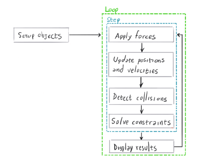
The diagram below provides a high-level overview of the typical process within a physics engine:

Vectors

A solid understanding of vectors and their operations is essential to grasping the inner workings of physics simulations. If you’re already comfortable with vector math, feel free to skip ahead. But if you need a refresher or are new to the concept, take a moment to review the appendix at the end of this article.

Particle Simulation

Particle simulation serves as a helpful starting point for understanding rigid body simulation. Simulating particles is simpler than simulating rigid bodies, and we can build upon the principles used for particle simulation to handle rigid bodies by introducing volume and shape to our particles. Plus, there’s a wealth of great particle physics engine tutorials available online, covering a wide range of scenarios and levels of realism/complexity.

A particle is, in essence, just a point in space defined by its position vector, its velocity vector, and its mass. As Newton’s First Law dictates, a particle’s velocity will only change if a force acts upon it. If the particle’s velocity vector has a non-zero length, its position will change over time.

To simulate a particle system, we begin by creating an array of particles, each initialized with a specific state. Each particle needs a fixed mass, a starting position in space, and an initial velocity. With our particles set up, we start the main simulation loop. In this loop, we perform the following calculations for each particle: determine the net force acting on it at that moment, update its velocity based on the acceleration produced by the force, and finally, update its position according to the newly calculated velocity.

The forces acting on a particle can arise from various sources depending on the type of simulation, including gravity, wind, magnetism, or a combination of these. A force can be global, such as the constant pull of gravity, or it can be a force that exists between particles, such as attraction or repulsion.

To achieve a realistic simulation speed, the time step we simulate should ideally match the actual time elapsed since the previous simulation step. However, we can manipulate this time step, scaling it up to make the simulation run faster or down to create a slow-motion effect.

Let’s say we have a particle with mass m, position p(_t_i), and velocity v(_t_i) at a specific point in time _t_i. A force f(_t_i) is applied to this particle at that instant. We can calculate the particle’s position, p(_t_i + 1), and velocity, v(_t_i + 1), at a future time _t_i + 1 using the following equations:

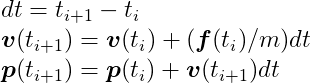
From a technical standpoint, we’re numerically integrating an ordinary differential equation that governs the particle’s motion. The method we’re using, the semi-implicit Euler method, is popular in game physics engines for its straightforward implementation and reasonable accuracy, especially when dealing with small time steps (dt). For a more in-depth look at the numerical methodology behind this method, the Differential Equation Basics lecture notes from the exceptional Physically Based Modeling: Principles and Practice course taught by Drs. Andy Witkin and David Baraff is an excellent resource.

Let’s illustrate this with a C language example of a simple particle simulation:

 1
 2
 3
 4
 5
 6
 7
 8
 9
10
11
12
13
14
15
16
17
18
19
20
21
22
23
24
25
26
27
28
29
30
31
32
33
34
35
36
37
38
39
40
41
42
43
44
45
46
47
48
49
50
51
52
53
54
55
56
57
58
59
60
61
62
63
64
65
66
67
68
69
70
71
72

#define NUM_PARTICLES 1

// Two dimensional vector.
typedef struct {
    float x;
    float y;
} Vector2;

// Two dimensional particle.
typedef struct {
    Vector2 position;
    Vector2 velocity;
    float mass;
} Particle;

// Global array of particles.
Particle particles[NUM_PARTICLES];

// Prints all particles' position to the output. We could instead draw them on screen
// in a more interesting application.
void  PrintParticles() {
    for (int i = 0; i < NUM_PARTICLES; ++i) {
        Particle *particle = &particles[i];
        printf("particle[%i] (%.2f, %.2f)\n", i, particle->position.x, particle->position.y);
    }
}

// Initializes all particles with random positions, zero velocities and 1kg mass.
void InitializeParticles() {
    for (int i = 0; i < NUM_PARTICLES; ++i) {
        particles[i].position = (Vector2){arc4random_uniform(50), arc4random_uniform(50)};
        particles[i].velocity = (Vector2){0, 0};
        particles[i].mass = 1;
    }
}

// Just applies Earth's gravity force (mass times gravity acceleration 9.81 m/s^2) to each particle.
Vector2 ComputeForce(Particle *particle) {
    return (Vector2){0, particle->mass * -9.81};
}

void RunSimulation() {
    float totalSimulationTime = 10; // The simulation will run for 10 seconds.
    float currentTime = 0; // This accumulates the time that has passed.
    float dt = 1; // Each step will take one second.
    
    InitializeParticles();
    PrintParticles();
    
    while (currentTime < totalSimulationTime) {
        // We're sleeping here to keep things simple. In real applications you'd use some
        // timing API to get the current time in milliseconds and compute dt in the beginning 
        // of every iteration like this:
        // currentTime = GetTime()
        // dt = currentTime - previousTime
        // previousTime = currentTime
        sleep(dt);

        for (int i = 0; i < NUM_PARTICLES; ++i) {
            Particle *particle = &particles[i];
            Vector2 force = ComputeForce(particle);
            Vector2 acceleration = (Vector2){force.x / particle->mass, force.y / particle->mass};
            particle->velocity.x += acceleration.x * dt;
            particle->velocity.y += acceleration.y * dt;
            particle->position.x += particle->velocity.x * dt;
            particle->position.y += particle->velocity.y * dt;
        }
        
        PrintParticles();
        currentTime += dt;
    }
}

If we call the RunSimulation function with a single particle, we’ll get an output similar to this:

 1
 2
 3
 4
 5
 6
 7
 8
 9
10
11

particle[0] (-8.00, 57.00)
particle[0] (-8.00, 47.19)
particle[0] (-8.00, 27.57)
particle[0] (-8.00, -1.86)
particle[0] (-8.00, -41.10)
particle[0] (-8.00, -90.15)
particle[0] (-8.00, -149.01)
particle[0] (-8.00, -217.68)
particle[0] (-8.00, -296.16)
particle[0] (-8.00, -384.45)
particle[0] (-8.00, -482.55)

As you can see, our particle began at position (-8, 57), and its y coordinate began to decrease at an increasing rate due to the downward acceleration caused by gravity.

To help visualize this, the following animation depicts three consecutive steps in the simulation of a single particle:

At the start, when t = 0, our particle is at position _p_0. After one step, it moves in the direction indicated by its velocity vector _v_0. In the next step, a force _f_1 is applied, causing the velocity vector to change as if the particle is being pulled in the direction of the force vector. In the subsequent steps, the direction of the force vector changes, but it continues to influence the particle’s upward motion.

Rigid Body Physics Simulation

In physics simulations, a rigid body is defined as a solid object that is incapable of deformation. While such perfectly rigid objects don’t exist in the real world – even the most durable materials will deform to some extent when subjected to force – the concept of a rigid body provides a useful model for game developers, simplifying the study of object dynamics in cases where we can disregard deformation.

A rigid body can be thought of as an extension of a particle. Like particles, rigid bodies possess mass, position, and velocity. However, unlike particles, rigid bodies have volume and shape, which means they can also rotate, adding layers of complexity, especially when working in three dimensions.

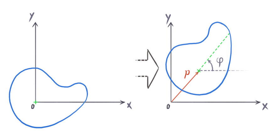
A rigid body naturally rotates around its center of mass, and we define a rigid body’s position as the position of its center of mass. When setting up a rigid body simulation, we typically initialize the rigid body with its center of mass at the origin and with a rotation angle of zero. Its position and rotation at any given time t will represent an offset from this initial state.

The center of mass represents the average position of the mass distribution within a body. Imagine a rigid body with mass M made up of N minuscule particles, each with mass _m_i and located at position _r_i within the body. We can calculate the center of mass using the following formula:

This formula illustrates that the center of mass is essentially the weighted average of the positions of all the particles, with the weights being their individual masses. If the body has a uniform density throughout, meaning its mass is evenly distributed, then the center of mass coincides with the body’s geometric center, also known as the centroid. As game physics engines typically work with the assumption of uniform density, we can use the geometric center as the center of mass.

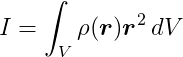
However, it’s important to remember that rigid bodies are not composed of a finite set of discrete particles; they are continuous. To account for this, we should ideally calculate the center of mass using an integral instead of a finite sum:

In this formula, r represents the position vector of each point within the body, and 𝜌 (rho) is a function that defines the density at any given point within the body. This integral, in essence, performs the same calculation as the finite sum but does so over the continuous volume V of the rigid body.

Since a rigid body can rotate, we need to introduce the concept of its angular properties. These properties mirror the linear properties we discussed for particles. In a two-dimensional space, a rigid body can only rotate around an axis perpendicular to the screen. This means we only need a single scalar value to represent its orientation. For this purpose, we typically use radians, which range from 0 to 2π for a full circle, rather than degrees (which range from 0 to 360 for a full circle), as radians simplify calculations.

For a rigid body to rotate, it requires angular velocity, a scalar quantity measured in radians per second, commonly denoted by the Greek letter ω (omega). However, to acquire angular velocity, the body needs to be acted upon by a rotational force, which we call torque, represented by the Greek letter τ (tau). We can express Newton’s Second Law in the context of rotation as follows:

In this equation, α (alpha) represents angular acceleration, and I represents the moment of inertia.

In the context of rotation, the moment of inertia is akin to mass for linear motion. It quantifies the resistance of a rigid body to changes in its angular velocity. In two dimensions, it’s a scalar value defined by the following formula:

Here, V indicates that we need to integrate over the entire volume of the body, r is the position vector of each point relative to the axis of rotation, _r_2 is simply the dot product of r with itself, and 𝜌 is a function that provides the density at each point within the body.

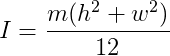
For instance, the moment of inertia of a 2-dimensional rectangular box with mass m, width w, and height h about its centroid is given by:

Here provides a comprehensive list of formulas for calculating the moment of inertia for various shapes about different axes.

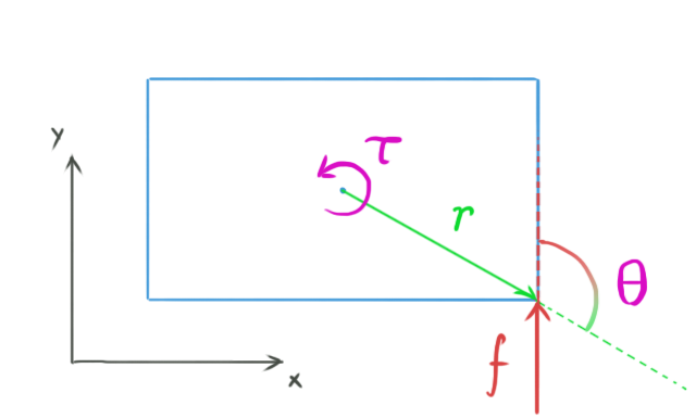
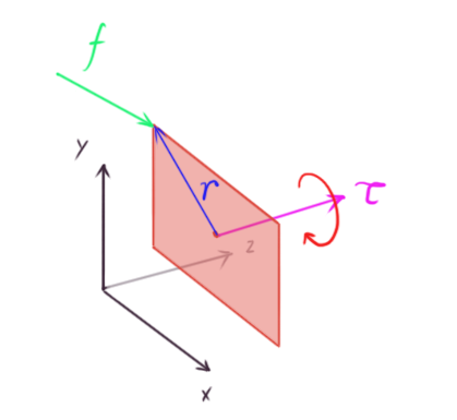
When a force is applied to a point on a rigid body, it can produce torque. In two dimensions, torque is a scalar quantity. The torque τ produced by a force f applied at a point on the body that has an offset vector r from the center of mass is calculated as:

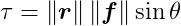
where θ (theta) represents the smallest angle between f and _r.

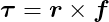
Interestingly, the formula for torque in two dimensions is identical to the formula for calculating the length of the cross product between r and _f. This means that in three dimensions, we can express torque as:

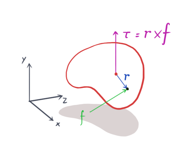
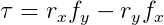
We can think of a two-dimensional simulation as a simplified case of a three-dimensional simulation. In this view, all rigid bodies are thin, flat objects existing and interacting within the xy-plane, with no movement along the z-axis. Consequently, both f and r will always lie in the xy-plane, resulting in a torque vector τ that always has zero x and y components (because the cross product is always perpendicular to the xy-plane). This means that τ will always be parallel to the z-axis, so only its z component truly matters. Therefore, we can simplify the calculation of torque in two dimensions to:

It’s remarkable how adding just one more dimension significantly increases the complexity. In three dimensions, we need a quaternion, a type of four-element vector, to represent the orientation of a rigid body. The moment of inertia becomes a 3x3 matrix known as the inertia tensor, which, unlike in two dimensions, is not constant. The inertia tensor depends on the rigid body’s orientation and changes over time as the body rotates. To delve into the intricacies of 3D rigid body simulation, Rigid Body Simulation I — Unconstrained Rigid Body Dynamics, another excellent resource from Witkin and Baraff’s Physically Based Modeling: Principles and Practice course, provides a comprehensive exploration of the topic.

The algorithm for simulating rigid bodies is quite similar to the one we used for particle simulation. The key difference is the addition of shape and rotational properties to our objects:

 1
 2
 3
 4
 5
 6
 7
 8
 9
10
11
12
13
14
15
16
17
18
19
20
21
22
23
24
25
26
27
28
29
30
31
32
33
34
35
36
37
38
39
40
41
42
43
44
45
46
47
48
49
50
51
52
53
54
55
56
57
58
59
60
61
62
63
64
65
66
67
68
69
70
71
72
73
74
75
76
77
78
79
80
81
82
83
84
85
86
87
88
89
90
91
92
93
94
95
96
97
98

#define NUM_RIGID_BODIES 1

// 2D box shape. Physics engines usually have a couple different classes of shapes
// such as circles, spheres (3D), cylinders, capsules, polygons, polyhedrons (3D)...
typedef struct {
    float width;
    float height;
    float mass;
    float momentOfInertia;
} BoxShape;

// Calculates the inertia of a box shape and stores it in the momentOfInertia variable.
void CalculateBoxInertia(BoxShape *boxShape) {
    float m = boxShape->mass;
    float w = boxShape->width;
    float h = boxShape->height;
    boxShape->momentOfInertia = m * (w * w + h * h) / 12;
}

// Two dimensional rigid body
typedef struct {
    Vector2 position;
    Vector2 linearVelocity;
    float angle;
    float angularVelocity;
    Vector2 force;
    float torque;
    BoxShape shape;
} RigidBody;

// Global array of rigid bodies.
RigidBody rigidBodies[NUM_RIGID_BODIES];

// Prints the position and angle of each body on the output.
// We could instead draw them on screen.
void PrintRigidBodies() {
    for (int i = 0; i < NUM_RIGID_BODIES; ++i) {
        RigidBody *rigidBody = &rigidBodies[i];
        printf("body[%i] p = (%.2f, %.2f), a = %.2f\n", i, rigidBody->position.x, rigidBody->position.y, rigidBody->angle);
    }
}

// Initializes rigid bodies with random positions and angles and zero linear and angular velocities.
// They're all initialized with a box shape of random dimensions.
void InitializeRigidBodies() {
    for (int i = 0; i < NUM_RIGID_BODIES; ++i) {
        RigidBody *rigidBody = &rigidBodies[i];
        rigidBody->position = (Vector2){arc4random_uniform(50), arc4random_uniform(50)};
        rigidBody->angle = arc4random_uniform(360)/360.f * M_PI * 2;
        rigidBody->linearVelocity = (Vector2){0, 0};
        rigidBody->angularVelocity = 0;
        
        BoxShape shape;
        shape.mass = 10;
        shape.width = 1 + arc4random_uniform(2);
        shape.height = 1 + arc4random_uniform(2);
        CalculateBoxInertia(&shape);
        rigidBody->shape = shape;
    }
}

// Applies a force at a point in the body, inducing some torque.
void ComputeForceAndTorque(RigidBody *rigidBody) {
    Vector2 f = (Vector2){0, 100};
    rigidBody->force = f;
    // r is the 'arm vector' that goes from the center of mass to the point of force application
    Vector2 r = (Vector2){rigidBody->shape.width / 2, rigidBody->shape.height / 2};
    rigidBody->torque = r.x * f.y - r.y * f.x;
}

void RunRigidBodySimulation() {
    float totalSimulationTime = 10; // The simulation will run for 10 seconds.
    float currentTime = 0; // This accumulates the time that has passed.
    float dt = 1; // Each step will take one second.
    
    InitializeRigidBodies();
    PrintRigidBodies();
    
    while (currentTime < totalSimulationTime) {
        sleep(dt);
        
        for (int i = 0; i < NUM_RIGID_BODIES; ++i) {
            RigidBody *rigidBody = &rigidBodies[i];
            ComputeForceAndTorque(rigidBody);
            Vector2 linearAcceleration = (Vector2){rigidBody->force.x / rigidBody->shape.mass, rigidBody->force.y / rigidBody->shape.mass};
            rigidBody->linearVelocity.x += linearAcceleration.x * dt;
            rigidBody->linearVelocity.y += linearAcceleration.y * dt;
            rigidBody->position.x += rigidBody->linearVelocity.x * dt;
            rigidBody->position.y += rigidBody->linearVelocity.y * dt;
            float angularAcceleration = rigidBody->torque / rigidBody->shape.momentOfInertia;
            rigidBody->angularVelocity += angularAcceleration * dt;
            rigidBody->angle += rigidBody->angularVelocity * dt;
        }
        
        PrintRigidBodies();
        currentTime += dt;
    }
}

When we call the RunRigidBodySimulation function for a single rigid body, it will output the body’s position and angle:

 1
 2
 3
 4
 5
 6
 7
 8
 9
10
11

body[0] p = (36.00, 12.00), a = 0.28
body[0] p = (36.00, 22.00), a = 15.28
body[0] p = (36.00, 42.00), a = 45.28
body[0] p = (36.00, 72.00), a = 90.28
body[0] p = (36.00, 112.00), a = 150.28
body[0] p = (36.00, 162.00), a = 225.28
body[0] p = (36.00, 222.00), a = 315.28
body[0] p = (36.00, 292.00), a = 420.28
body[0] p = (36.00, 372.00), a = 540.28
body[0] p = (36.00, 462.00), a = 675.28
body[0] p = (36.00, 562.00), a = 825.28

Because we’re applying an upward force of 100 Newtons, only the y-coordinate changes. Since this force isn’t directly applied to the center of mass, it creates torque, causing the body to rotate counterclockwise, as indicated by the increasing rotation angle.

Visually, the simulation looks similar to the particle animation, but now we have shapes moving and rotating within our simulated environment.

This type of simulation is considered unconstrained because the bodies are free to move without any restrictions. They don’t interact or collide with each other. While illustrative, simulations without collisions are not particularly exciting or useful. In the next part of this series, we’ll delve into the world of collision detection and explore techniques for resolving collisions once they’re detected.

Appendix: Vectors

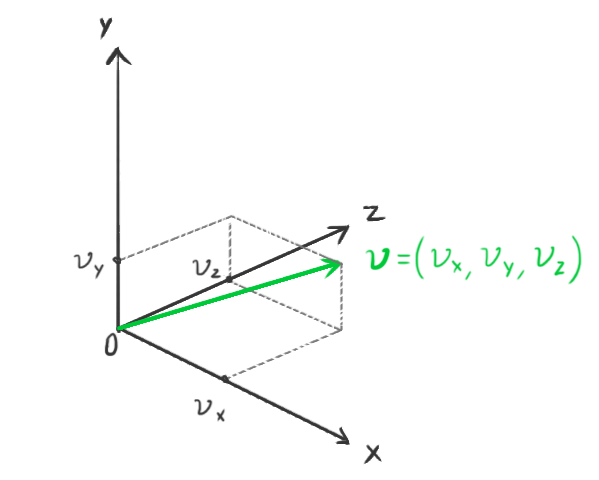
A vector is a mathematical entity characterized by its length (or more formally, its magnitude) and direction. We can visualize vectors intuitively in the Cartesian coordinate system. In two dimensions, we decompose a vector into its x and y components, while in three dimensions, we use the x, y, and z components.

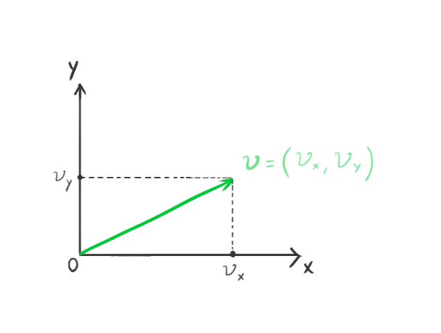
We represent vectors using bold lowercase letters. The components of a vector are represented by the same letter in regular typeface, along with a subscript indicating the corresponding component. For example:

represents a two-dimensional vector. Each component of the vector corresponds to the distance from the origin along the respective coordinate axis.

Physics engines commonly incorporate their own lightweight, optimized math libraries. The Bullet Physics engine, for example, has a separate math library called Linear Math, which can be used independently without relying on Bullet’s physics simulation features. This library includes classes for representing vectors, matrices, and other mathematical entities. It’s designed to take advantage of SIMD instructions if they are available on the system.

Let’s review some of the fundamental algebraic operations that we can perform on vectors.

Length

We use the || || symbol to represent the length, or magnitude, operator. The length of a vector can be calculated from its components using the well-known Pythagorean theorem theorem for right triangles. For a two-dimensional vector, the length is:

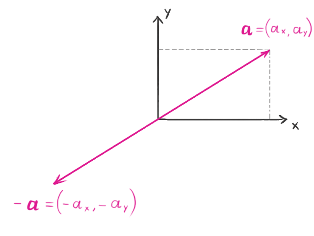
Negation

Negating a vector doesn’t change its length, but it reverses its direction. For instance, if we have the vector:

its negation would be:

Addition and Subtraction

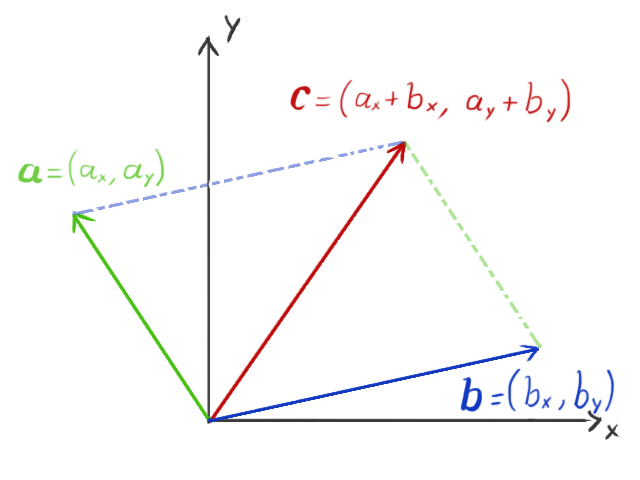
We can add or subtract vectors. Subtracting two vectors is equivalent to adding one vector to the negation of the other. To add or subtract vectors, we simply add or subtract their corresponding components:

We can visualize the resulting vector as pointing to the same point we would reach if we placed the two original vectors end-to-end:

Scalar Multiplication

Multiplying a vector by a scalar, which for our purposes is any real number, scales the length of the vector by that amount. If the scalar is negative, the direction of the vector is also reversed.

Dot Product

The dot product is an operation that takes two vectors as input and produces a scalar value as output. It is defined as:

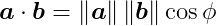
where ø represents the angle between the two vectors. From a computational perspective, it’s easier to calculate the dot product using the components of the vectors:

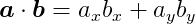
The dot product is equivalent to the length of the projection of vector a onto vector b multiplied by the length of _b. We can reverse this, taking the length of the projection of b onto a and multiplying by the length of a to obtain the same result. This means that the dot product is commutative – the dot product of a with b is the same as the dot product of b with a. One useful property of the dot product is that if the two vectors are orthogonal (the angle between them is 90 degrees), the dot product is zero because cos 90 = 0.

Cross Product

In three-dimensional space, we can also multiply two vectors to produce another vector using the cross product. The cross product is defined as:

and the length of the cross product is given by:

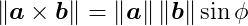
Here, ø represents the smaller angle between vectors a and _b. The resulting vector c is perpendicular to both a and _b. If a and b are parallel, meaning the angle between them is either zero or 180 degrees, then c will be the zero vector because sin 0 = sin 180 = 0.

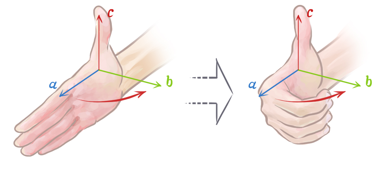
Unlike the dot product, the cross product is not commutative. The order of the vectors in the cross product matters:

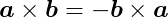
We can determine the direction of the resulting vector using the right-hand rule. To do this, open your right hand, point your index finger in the direction of a, and orient your hand so that when you make a fist, your fingers move directly towards b through the smallest angle between the two vectors. Your thumb will then be pointing in the direction of a × _b.