TensorFlow, an open-source software library developed by Google, is widely used for building machine learning and deep learning systems. These systems utilize advanced algorithms to enable computers to identify intricate patterns and make optimal decisions automatically.

For a deeper understanding of these systems, we recommend exploring the Toptal blog posts on machine learning and deep learning.

At its core, TensorFlow is a library designed for dataflow programming. It employs various optimization techniques to simplify and accelerate the calculation of mathematical expressions.

TensorFlow’s key features include:

• Efficient handling of mathematical expressions involving multi-dimensional arrays
• Strong support for deep neural networks and machine learning concepts
• GPU/CPU computing capabilities, allowing code execution on both architectures
• High scalability of computation across multiple machines and massive datasets

These features collectively make TensorFlow an ideal framework for implementing machine intelligence at a production level.

This TensorFlow tutorial will guide you on utilizing simple yet effective machine learning methods within TensorFlow. You’ll also learn how to leverage its auxiliary libraries for debugging, visualizing, and fine-tuning the models you create.

Setting Up TensorFlow

We’ll be working with the TensorFlow Python API, compatible with Python 2.7 and Python 3.3+. The GPU version (Linux exclusive) necessitates the Cuda Toolkit 7.0+ and cuDNN v2+.

To install TensorFlow, we’ll utilize the Conda package manager. Conda enables us to maintain separate environments on a machine. For instructions on installing Conda, refer to here.

Once Conda is installed, we can create our environment for TensorFlow installation and usage. The following command will set up our environment with additional libraries like NumPy, which proves highly beneficial when working with TensorFlow.

This environment will have Python version 2.7 installed, which we’ll be using throughout this article.

1

conda create --name TensorflowEnv biopython

For simplicity, we’re installing biopython instead of just NumPy. This includes NumPy and other essential packages. You can install packages as needed using conda install or pip install.

Let’s activate the created Conda environment:

1

source activate TensorFlowEnv 

This allows us to utilize packages within this environment without interfering with globally installed packages or those in other environments.

The pip installation tool, a standard component of a Conda environment, will be used to install the TensorFlow library. It’s recommended to update pip to the latest version first:

1

pip install --upgrade pip

Now, we can proceed with installing TensorFlow:

1

pip install tensorflow

Downloading and building TensorFlow may take a while. At the time of writing, this installs TensorFlow 1.1.0.

Understanding Data Flow Graphs

TensorFlow represents computations using data flow graphs. Each node in the graph denotes an instance of a mathematical operation (e.g., addition, division, multiplication), while each edge represents a multi-dimensional dataset (tensor) on which these operations are performed.

TensorFlow’s computation graphs are managed structures where each node embodies an operation. Each operation can have zero or more inputs and outputs.

Edges in TensorFlow fall into two categories: Normal edges carry data structures (tensors), potentially serving as input for other operations. Special edges govern the dependency between nodes, dictating the order of operations—one node might wait for another to complete.

Exploring Simple Expressions

Before delving deeper into TensorFlow’s components, let’s work through a session to understand the structure of a TensorFlow program.

We’ll start with a simple expression. Suppose we want to evaluate the function y = 5*x + 13 using TensorFlow.

In standard Python code, it would look like this:

1
2
3

x = -2.0
y = 5*x + 13
print y

which, in this case, yields 3.0.

Now, let’s translate this expression into TensorFlow.

Constants

TensorFlow uses the constant function to create constants. Its signature is constant(value, dtype=None, shape=None, name='Const', verify_shape=False). Here, value represents the constant’s value used in computations, dtype specifies the data type (e.g., float32/64, int8/16), shape defines optional dimensions, name provides an optional name for the tensor, and the last parameter is a boolean indicating whether to verify the shape of values.

To define constants with specific values within your training model, use the constant object as follows:

1

z = tf.constant(5.2, name="x", dtype=tf.float32)

Variables

Variables in TensorFlow are in-memory buffers holding tensors. They require explicit initialization and in-graph usage to maintain state across sessions. Calling the constructor adds the variable to the computational graph.

Variables are particularly valuable when training models, as they store and update parameters. The initial value passed as a constructor argument represents a tensor or an object convertible to a tensor. To initialize a variable with predefined or random values for training and subsequent updates over iterations, define it like this:

1

k = tf.Variable(tf.zeros([1]), name="k")

Alternatively, you can use non-trainable variables in calculations:

1

k = tf.Variable(tf.add(a, b), trainable=False)

Sessions

To evaluate nodes, we execute the computational graph within a session.

A session manages the control and state of the TensorFlow runtime. Without parameters, it utilizes the default graph created in the current session. The session class also accepts a graph parameter, specifying the graph to be executed within that session.

The code snippet below demonstrates how the terms defined above can be used in TensorFlow to calculate a simple linear function:

 1
 2
 3
 4
 5
 6
 7
 8
 9
10
11
12
13

import tensorflow as tf

x = tf.constant(-2.0, name="x", dtype=tf.float32)
a = tf.constant(5.0, name="a", dtype=tf.float32)
b = tf.constant(13.0, name="b", dtype=tf.float32)

y = tf.Variable(tf.add(tf.multiply(a, x), b))

init = tf.global_variables_initializer()

with tf.Session() as session:
    session.run(init)
    print session.run(y)

Working with TensorFlow: Defining Computational Graphs

Dataflow graphs offer the advantage of separating the execution model from its actual execution (on CPU, GPU, or a combination). Once implemented, TensorFlow software can run on CPUs or GPUs, abstracting away the complexities of code execution.

The computation graph is implicitly built as you use the TensorFlow library, without explicitly instantiating Graph objects.

A simple line of code like c = tf.add(a, b) creates a Graph object in TensorFlow. This generates an operation node taking tensors a and b as input and producing their sum c as output.

This implicit graph construction eliminates the need to directly call the graph object. A TensorFlow graph object comprises operations and tensors, with tensors acting as data units between operations. Multiple graphs can coexist, each assigned to a different session. For instance, c = tf.add(a, b) creates an operation node that takes tensors a and b and outputs their sum c.

TensorFlow also provides a feed mechanism to inject tensor values into any operation within the graph. This feed data replaces the operation’s output with the provided tensor value and is passed as an argument to the run() function call.

Placeholders offer a way to inject data into the computation graph. These placeholders are bound within expressions. The signature for a placeholder is:

1

placeholder(dtype, shape=None, name=None)

where dtype specifies the tensor elements’ data type, and you can optionally provide the tensor’s shape and a name for the operation.

If no shape is provided, the tensor can accept any shape. However, placeholder tensors must be fed with data; otherwise, an error occurs during session execution if data is missing:

1

InvalidArgumentError (see above for traceback): You must feed a value for placeholder tensor 'y' with dtype float

Placeholders empower developers to define operations and the computational graph without upfront data. Data can be supplied dynamically during runtime from external sources.

Let’s illustrate this with a simple example of multiplying two integers, x and y, using TensorFlow. We’ll use a placeholder and the feed mechanism through the session’s run method.

1
2
3
4
5
6
7
8
9

import tensorflow as tf

x = tf.placeholder(tf.float32, name="x")
y = tf.placeholder(tf.float32, name="y")

z = tf.multiply(x, y, name="z")

with tf.Session() as session:
    print session.run(z, feed_dict={x: 2.1, y: 3.0})

Visualizing the Computational Graph with TensorBoard

TensorBoard is a visualization tool for analyzing data flow graphs, aiding in understanding machine learning models.

It provides insights into various statistics related to parameters and details about the computational graph’s components. Deep neural networks often involve numerous nodes, and TensorBoard helps developers understand each node’s role and how computations flow during TensorFlow runtime.

Let’s revisit our linear function example (y = a*x + b) from earlier in this tutorial.

To log session events for TensorBoard visualization, TensorFlow offers the FileWriter class. This class creates an event file to store summaries. Its constructor takes six parameters:

1

__init__(logdir, graph=None, max_queue=10, flush_secs=120, graph_def=None, filename_suffix=None)

The logdir parameter is mandatory, while others have default values. The graph parameter is taken from the session object created in the training program. Here’s the complete example code:

 1
 2
 3
 4
 5
 6
 7
 8
 9
10
11
12
13
14
15
16
17
18
19
20
21

import tensorflow as tf


x = tf.constant(-2.0, name="x", dtype=tf.float32)
a = tf.constant(5.0, name="a", dtype=tf.float32)
b = tf.constant(13.0, name="b", dtype=tf.float32)


y = tf.Variable(tf.add(tf.multiply(a, x), b))


init = tf.global_variables_initializer()


with tf.Session() as session:
    merged = tf.summary.merge_all() // new
    writer = tf.summary.FileWriter("logs", session.graph) // new


    session.run(init)
    print session.run(y)

We’ve added two lines: one to merge summaries from the default graph and another to utilize FileWriter for dumping events to the file.

After running the program, an event file is generated in the logs directory. Now, let’s run TensorBoard:

1

tensorboard --logdir logs/

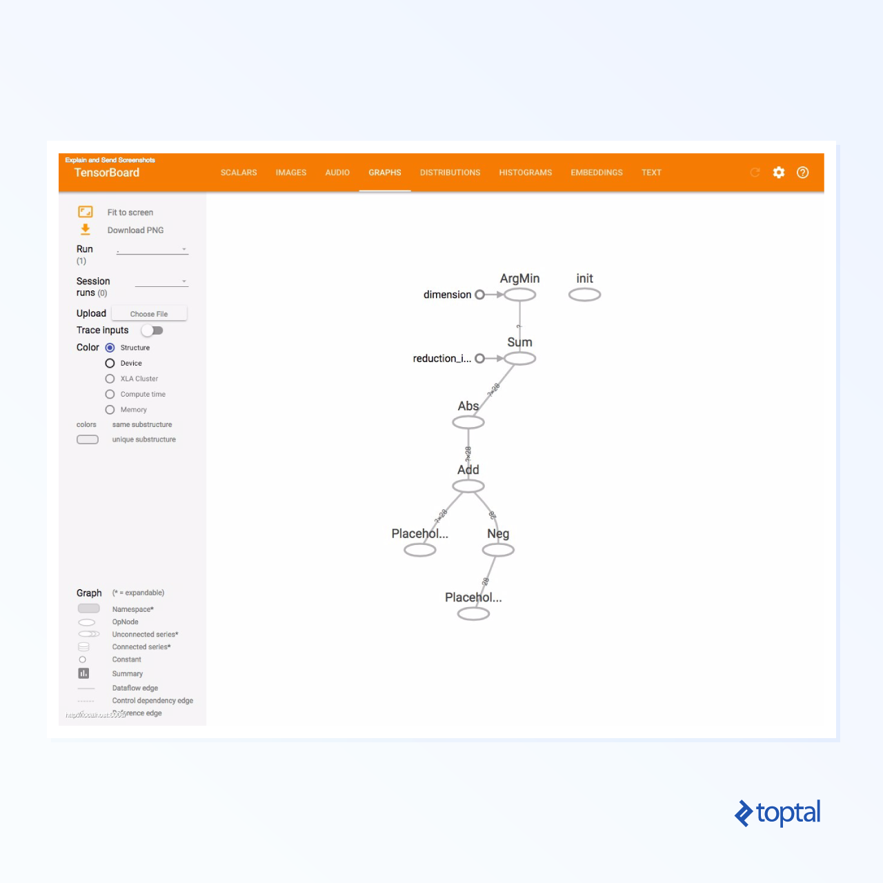
TensorBoard will start on the default port 6006. Open http://localhost:6006 in your web browser, and navigate to the “Graphs” menu item to visualize the graph, similar to the image below:

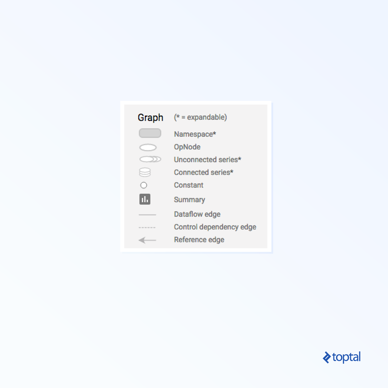
TensorBoard uses distinct symbols for constants and summary nodes, as detailed below:

Mathematics in TensorFlow

Tensors are the fundamental data structures in TensorFlow, representing the connecting edges within a dataflow graph.

A tensor is essentially a multidimensional array or list characterized by three parameters: rank, shape, and type.

• Rank: Represents the number of dimensions in the tensor, also referred to as the order or n-dimensions. For instance, a rank 1 tensor is a vector, and a rank 2 tensor is a matrix.
• Shape: Defines the number of rows and columns in the tensor.
• Type: Specifies the data type assigned to tensor elements.

To create a tensor in TensorFlow, you can build an n-dimensional array using libraries like NumPy or by converting a Python n-dimensional array into a TensorFlow tensor.

Let’s create a 1-dimensional tensor using a NumPy array, which we’ll construct from a Python list:

1
2

import numpy as np
tensor_1d = np.array([1.45, -1, 0.2, 102.1])

Working with this array is similar to using a Python list, but the NumPy array includes additional properties such as dimension, shape, and type.

 1
 2
 3
 4
 5
 6
 7
 8
 9
10
11
12
13
14
15
16
17

> > print tensor1d
[   1.45   -1.      0.2   102.1 ]

> > print tensor1d[0]
1.45

> > print tensor1d[2]
0.2

> > print tensor1d.ndim
1

> > print tensor1d.shape
(4,)

> > print tensor1d.dtype
float64

Converting a NumPy array to a TensorFlow tensor is straightforward using the [convert\_to\_tensor](https://www.tensorflow.org/api_docs/python/tf/convert_to_tensor) function. This function converts Python objects like tensor objects, NumPy arrays, Python lists, and scalars into tensor objects.

1

tensor = tf.convert_to_tensor(tensor_1d, dtype=tf.float64)

By binding our tensor to a TensorFlow session, we can see the results of the conversion:

1
2
3
4
5
6

tensor = tf.convert_to_tensor(tensor_1d, dtype=tf.float64)

with tf.Session() as session:
    print session.run(tensor)
    print session.run(tensor[0])
    print session.run(tensor[1])

Output:

1
2
3

[   1.45   -1.      0.2   102.1 ]
1.45
-1.0

Creating a 2-dimensional tensor (a matrix) follows a similar approach:

 1
 2
 3
 4
 5
 6
 7
 8
 9
10
11
12
13
14
15

tensor_2d = np.array(np.random.rand(4, 4), dtype='float32')
tensor_2d_1 = np.array(np.random.rand(4, 4), dtype='float32')
tensor_2d_2 = np.array(np.random.rand(4, 4), dtype='float32')

m1 = tf.convert_to_tensor(tensor_2d)
m2 = tf.convert_to_tensor(tensor_2d_1)
m3 = tf.convert_to_tensor(tensor_2d_2)
mat_product = tf.matmul(m1, m2)
mat_sum = tf.add(m2, m3)
mat_det = tf.matrix_determinant(m3)

with tf.Session() as session:
    print session.run(mat_product)
    print session.run(mat_sum)
    print session.run(mat_det)

Tensor Operations

The examples above introduce TensorFlow operations performed on vectors and matrices. These operations carry out specific calculations on the tensors, as summarized in the table below:

These TensorFlow operations work element-wise on tensor objects. For instance, to calculate the cosine of a vector x, the TensorFlow operation performs calculations for each element in the provided tensor.

1
2
3
4

tensor_1d = np.array([0, 0, 0])
tensor = tf.convert_to_tensor(tensor_1d, dtype=tf.float64)
with tf.Session() as session:
    print session.run(tf.cos(tensor))

Output:

1

[ 1.  1.  1.]

Matrix Operations

Matrix operations are crucial in machine learning models, especially linear regression, where they are frequently employed. TensorFlow supports common matrix operations such as multiplication, transposing, inversion, calculating the determinant, solving linear equations, and many more.

Let’s explore some basic matrix operations like multiplication, retrieving the transpose, calculating the determinant, and more.

Below are examples demonstrating these operations:

 1
 2
 3
 4
 5
 6
 7
 8
 9
10
11
12
13
14
15
16
17
18
19
20
21
22
23
24

import tensorflow as tf
import numpy as np

def convert(v, t=tf.float32):
    return tf.convert_to_tensor(v, dtype=t)

m1 = convert(np.array(np.random.rand(4, 4), dtype='float32'))
m2 = convert(np.array(np.random.rand(4, 4), dtype='float32'))
m3 = convert(np.array(np.random.rand(4, 4), dtype='float32'))
m4 = convert(np.array(np.random.rand(4, 4), dtype='float32'))
m5 = convert(np.array(np.random.rand(4, 4), dtype='float32'))

m_tranpose = tf.transpose(m1)
m_mul = tf.matmul(m1, m2)
m_det = tf.matrix_determinant(m3)
m_inv = tf.matrix_inverse(m4)
m_solve = tf.matrix_solve(m5, [[1], [1], [1], [1]])

with tf.Session() as session:
    print session.run(m_tranpose)
    print session.run(m_mul)
    print session.run(m_inv)
    print session.run(m_det)
    print session.run(m_solve)

Data Transformation

Reduction

TensorFlow supports various reduction operations, which remove one or more dimensions from a tensor by performing calculations across those dimensions. A list of supported reductions can be found in the TensorFlow documentation. We’ll illustrate a few below.

 1
 2
 3
 4
 5
 6
 7
 8
 9
10
11
12
13
14
15
16
17
18
19
20
21
22
23
24
25
26
27
28
29
30
31
32
33
34
35
36
37
38
39
40
41
42
43
44
45
46
47
48
49
50
51
52
53
54
55
56
57
58
59

import tensorflow as tf
import numpy as np

def convert(v, t=tf.float32):
    return tf.convert_to_tensor(v, dtype=t)

x = convert(
    np.array(
        [
            (1, 2, 3),
            (4, 5, 6),
            (7, 8, 9)
        ]), tf.int32)

bool_tensor = convert([(True, False, True), (False, False, True), (True, False, False)], tf.bool)

red_sum_0 = tf.reduce_sum(x)
red_sum = tf.reduce_sum(x, axis=1)

red_prod_0 = tf.reduce_prod(x)
red_prod = tf.reduce_prod(x, axis=1)

red_min_0 = tf.reduce_min(x)
red_min = tf.reduce_min(x, axis=1)

red_max_0 = tf.reduce_max(x)
red_max = tf.reduce_max(x, axis=1)

red_mean_0 = tf.reduce_mean(x)
red_mean = tf.reduce_mean(x, axis=1)

red_bool_all_0 = tf.reduce_all(bool_tensor)
red_bool_all = tf.reduce_all(bool_tensor, axis=1)

red_bool_any_0 = tf.reduce_any(bool_tensor)
red_bool_any = tf.reduce_any(bool_tensor, axis=1)


with tf.Session() as session:
    print "Reduce sum without passed axis parameter: ", session.run(red_sum_0)
    print "Reduce sum with passed axis=1: ", session.run(red_sum)

    print "Reduce product without passed axis parameter: ", session.run(red_prod_0)
    print "Reduce product with passed axis=1: ", session.run(red_prod)

    print "Reduce min without passed axis parameter: ", session.run(red_min_0)
    print "Reduce min with passed axis=1: ", session.run(red_min)

    print "Reduce max without passed axis parameter: ", session.run(red_max_0)
    print "Reduce max with passed axis=1: ", session.run(red_max)

    print "Reduce mean without passed axis parameter: ", session.run(red_mean_0)
    print "Reduce mean with passed axis=1: ", session.run(red_mean)

    print "Reduce bool all without passed axis parameter: ", session.run(red_bool_all_0)
    print "Reduce bool all with passed axis=1: ", session.run(red_bool_all)

    print "Reduce bool any without passed axis parameter: ", session.run(red_bool_any_0)
    print "Reduce bool any with passed axis=1: ", session.run(red_bool_any)

Output:

 1
 2
 3
 4
 5
 6
 7
 8
 9
10
11
12
13
14

Reduce sum without passed axis parameter:  45
Reduce sum with passed axis=1:  [ 6 15 24]
Reduce product without passed axis parameter:  362880
Reduce product with passed axis=1:  [  6 120 504]
Reduce min without passed axis parameter:  1
Reduce min with passed axis=1:  [1 4 7]
Reduce max without passed axis parameter:  9
Reduce max with passed axis=1:  [3 6 9]
Reduce mean without passed axis parameter:  5
Reduce mean with passed axis=1:  [2 5 8]
Reduce bool all without passed axis parameter:  False
Reduce bool all with passed axis=1:  [False False False]
Reduce bool any without passed axis parameter:  True
Reduce bool any with passed axis=1:  [ True  True  True]

Reduction operators take the tensor to be reduced as the first parameter. The second, optional parameter specifies the dimensions along which to perform the reduction. If omitted, the reduction applies to all dimensions.

Consider the [reduce\_sum](https://www.tensorflow.org/api_docs/python/tf/math/reduce_sum) operation. We pass a 2-dimensional tensor and reduce it along dimension 1.

The resulting sum would be:

1

[1 + 2 + 3 = 6, 4 + 5 + 6 = 15, 7 + 8 + 9 = 24]

If we reduced along dimension 0 instead:

1

[1 + 4 + 7 = 12, 2 + 5 + 8 = 15, 3 + 6 + 9 = 18]

Without specifying an axis, the result is the overall sum:

1

1 + 4 + 7 = 12, 2 + 5 + 8 = 15, 3 + 6 + 9 = 45

All reduction functions share a similar interface and are listed in the TensorFlow reduction documentation.

Segmentation

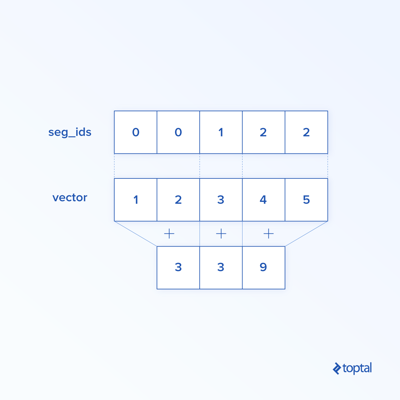
Segmentation maps dimensions onto provided segment indices, grouping elements under repeated indices. The resulting elements are determined by an index row.

For example, we have segmented IDs: [0, 0, 1, 2, 2] applied on tensor tens1, meaning that the first and second arrays will be transformed following segmentation operation (in our case summation) and will get a new array, which looks like (2, 8, 1, 0) = (2+0, 5+3, 3-2, -5+5). The third element in tensor tens1 is untouched because it isn’t grouped in any repeated index, and last two arrays are summed in same way as it was the case for the first group. Beside summation, TensorFlow supports product, mean, max, and min`.

 1
 2
 3
 4
 5
 6
 7
 8
 9
10
11
12
13
14
15
16
17
18
19
20
21
22

import tensorflow as tf
import numpy as np




def convert(v, t=tf.float32):
    return tf.convert_to_tensor(v, dtype=t)


seg_ids = tf.constant([0, 0, 1, 2, 2])
tens1 = convert(np.array([(2, 5, 3, -5), (0, 3, -2, 5), (4, 3, 5, 3), (6, 1, 4, 0), (6, 1, 4, 0)]), tf.int32)
tens2 = convert(np.array([1, 2, 3, 4, 5]), tf.int32)


seg_sum = tf.segment_sum(tens1, seg_ids)
seg_sum_1 = tf.segment_sum(tens2, seg_ids)


with tf.Session() as session:
    print "Segmentation sum tens1: ", session.run(seg_sum)
    print "Segmentation sum tens2: ", session.run(seg_sum_1)

1
2
3
4
5
6

Segmentation sum tens1:  
[[ 2  8  1  0]
 [ 4  3  5  3]
 [12  2  8  0]]
 
Segmentation sum tens2: [3 3 9]

Sequence Utilities

Sequence utilities include functions like:

• [argmin](https://www.tensorflow.org/api_docs/python/tf/math/argmin): Returns the index with the minimum value across tensor axes.
• [argmax](https://www.tensorflow.org/api_docs/python/tf/math/argmax): Returns the index with the maximum value across tensor axes.
• [setdiff](https://www.tensorflow.org/api_docs/python/tf/sets/difference): Computes the difference between two lists of numbers or strings.
• [where](https://www.tensorflow.org/api_docs/python/tf/where): Returns elements from either of two input elements (x or y) based on a condition.
• [unique](https://www.tensorflow.org/api_docs/python/tf/unique): Returns unique elements in a 1-dimensional tensor.

Here are some examples:

 1
 2
 3
 4
 5
 6
 7
 8
 9
10
11
12
13
14
15
16
17
18
19
20
21
22
23
24
25
26
27
28
29
30
31
32

import numpy as np
import tensorflow as tf

def convert(v, t=tf.float32):
    return tf.convert_to_tensor(v, dtype=t)

x = convert(np.array([
    [2, 2, 1, 3],
    [4, 5, 6, -1],
    [0, 1, 1, -2],
    [6, 2, 3, 0]
]))

y = convert(np.array([1, 2, 5, 3, 7]))
z = convert(np.array([1, 0, 4, 6, 2]))

arg_min = tf.argmin(x, 1)
arg_max = tf.argmax(x, 1)
unique = tf.unique(y)
diff = tf.setdiff1d(y, z)

with tf.Session() as session:
    print "Argmin = ", session.run(arg_min)
    print "Argmax = ", session.run(arg_max)

    print "Unique_values = ", session.run(unique)[0]
    print "Unique_idx = ", session.run(unique)[1]

    print "Setdiff_values = ", session.run(diff)[0]
    print "Setdiff_idx = ", session.run(diff)[1]

    print session.run(diff)[1]

Output:

1
2
3
4
5
6

Argmin = [2 3 3 3]
Argmax =  [3 2 1 0]
Unique_values =  [ 1.  2.  5.  3.  7.]
Unique_idx =  [0 1 2 3 4]
Setdiff_values =  [ 5.  3.  7.]
Setdiff_idx =  [2 3 4]

Machine Learning with TensorFlow

Let’s explore machine learning use cases with TensorFlow. Our first example implements a data classification algorithm using the kNN approach, while the second uses linear regression algorithm.

kNN

k-Nearest Neighbors (kNN) is a supervised learning algorithm that classifies data based on distance metrics, such as Euclidean distance, against a training dataset. Despite its simplicity, kNN is powerful for data classification.

Pros:

• High accuracy with a sufficiently large training model.
• Robust to outliers, requiring no assumptions about the data distribution.

Cons:

• Computationally expensive.
• Memory-intensive, as new data points must be compared to all training instances.

We’ll use Euclidean distance, which calculates the distance between two points as follows:

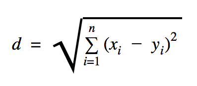
where n is the number of dimensions, x represents the training data vector, and y is the new data point to classify.

 1
 2
 3
 4
 5
 6
 7
 8
 9
10
11
12
13
14
15
16
17
18
19
20
21
22
23
24
25
26
27
28
29
30
31
32
33
34
35
36
37
38
39
40
41
42
43
44
45
46
47
48
49

import os
import numpy as np
import tensorflow as tf

ccf_train_data = "train_dataset.csv"
ccf_test_data = "test_dataset.csv"

dataset_dir = os.path.abspath(os.path.join(os.path.dirname(__file__), '../datasets'))

ccf_train_filepath = os.path.join(dataset_dir, ccf_train_data)
ccf_test_filepath = os.path.join(dataset_dir, ccf_test_data)

def load_data(filepath):
    from numpy import genfromtxt

    csv_data = genfromtxt(filepath, delimiter=",", skip_header=1)
    data = []
    labels = []

    for d in csv_data:
        data.append(d[:-1])
        labels.append(d[-1])

    return np.array(data), np.array(labels)

train_dataset, train_labels = load_data(ccf_train_filepath)
test_dataset, test_labels = load_data(ccf_test_filepath)

train_pl = tf.placeholder("float", [None, 28])
test_pl = tf.placeholder("float", [28])

knn_prediction = tf.reduce_sum(tf.abs(tf.add(train_pl, tf.negative(test_pl))), axis=1)

pred = tf.argmin(knn_prediction, 0)

with tf.Session() as tf_session:
    missed = 0

    for i in xrange(len(test_dataset)):
        knn_index = tf_session.run(pred, feed_dict={train_pl: train_dataset, test_pl: test_dataset[i]})

        print "Predicted class {} -- True class {}".format(train_labels[knn_index], test_labels[i])

        if train_labels[knn_index] != test_labels[i]:
            missed += 1

    tf.summary.FileWriter("../samples/article/logs", tf_session.graph)

print "Missed: {} -- Total: {}".format(missed, len(test_dataset))

The dataset used in this example is available in the Kaggle datasets section. We’ll be working with the one dataset, which contains credit card transactions made by European cardholders. We’ll use the raw data without any preprocessing. This dataset is known to be highly unbalanced, according to its Kaggle description. It includes 31 variables: Time, V1, …, V28, Amount, and Class. Our code sample focuses on V1, …, V28, and Class. The “Class” variable labels fraudulent transactions as 1 and non-fraudulent ones as 0.

The code primarily uses concepts explained earlier, except for the load_data(filepath) function, which reads a CSV file and returns a tuple containing data and corresponding labels defined in the CSV.

We define placeholders for test and training data. Training data is used by the prediction model to determine labels for input data requiring classification. In our kNN implementation, Euclidean distance identifies the nearest label.

The error rate is calculated by dividing the number of misclassifications by the total number of examples. In our case, the error rate is 0.2, indicating that the classifier misclassified 20% of the test data.

Linear Regression

Linear regression seeks a linear relationship between two variables. Given a dependent variable y and an independent variable x, the goal is to estimate the parameters of the function y = Wx + b.

Widely used in applied sciences, linear regression introduces two key machine learning concepts: Cost function and gradient descent method for finding function minima.

Machine learning algorithms employing this method aim to predict y values as a function of x. In linear regression, the unknowns W and b are determined during the training process. Typically, the mean square error serves as the cost function, and gradient descent acts as the optimization algorithm to locate a local minimum of the cost function.

While gradient descent finds local minima, it can be used to search for a global minimum by repeatedly starting from random points after finding a local minimum. With a limited number of minima and a sufficiently large number of attempts, there’s a good chance of finding the global minimum. We’ll delve deeper into this technique in a future article.

 1
 2
 3
 4
 5
 6
 7
 8
 9
10
11
12
13
14
15
16
17
18
19
20
21
22
23
24
25
26
27
28
29
30
31
32
33
34
35
36
37
38
39
40
41
42
43
44
45
46
47
48
49
50
51
52

import tensorflow as tf
import numpy as np

test_data_size = 2000
iterations = 10000
learn_rate = 0.005

def generate_test_values():
    train_x = []
    train_y = []

    for _ in xrange(test_data_size):
        x1 = np.random.rand()
        x2 = np.random.rand()
        x3 = np.random.rand()
        y_f = 2 * x1 + 3 * x2 + 7 * x3 + 4
        train_x.append([x1, x2, x3])
        train_y.append(y_f)

    return np.array(train_x), np.transpose([train_y])

x = tf.placeholder(tf.float32, [None, 3], name="x")
W = tf.Variable(tf.zeros([3, 1]), name="W")
b = tf.Variable(tf.zeros([1]), name="b")
y = tf.placeholder(tf.float32, [None, 1])

model = tf.add(tf.matmul(x, W), b)

cost = tf.reduce_mean(tf.square(y - model))
train = tf.train.GradientDescentOptimizer(learn_rate).minimize(cost)

train_dataset, train_values = generate_test_values()

init = tf.global_variables_initializer()

with tf.Session() as session:
    session.run(init)

    for _ in xrange(iterations):

        session.run(train, feed_dict={
            x: train_dataset,
            y: train_values
        })

    print "cost = {}".format(session.run(cost, feed_dict={
        x: train_dataset,
        y: train_values
    }))

    print "W = {}".format(session.run(W))
    print "b = {}".format(session.run(b))

Output:

1
2
3
4
5

cost = 3.1083032809e-05
W = [[ 1.99049103]
 [ 2.9887135 ]
 [ 6.98754263]]
b = [ 4.01742554]

This example introduces two new variables, cost and train, defining the optimizer and the function to minimize.

Ideally, the resulting W and b parameters should match those defined in the generate_test_values function. Line 17 defines the function for generating linear data points for training, with w1=2, w2=3, w3=7, and b=4. This example demonstrates multivariate linear regression, using multiple independent variables.

Conclusion

This TensorFlow tutorial highlights the framework’s power in simplifying work with mathematical expressions and multi-dimensional arrays, which are fundamental to machine learning. TensorFlow also abstracts away the complexities of executing data graphs and scaling computations.

TensorFlow’s popularity has surged, finding applications in image recognition, video detection, text processing (like sentiment analysis), and more. While grasping TensorFlow’s core concepts may take time, its documentation and community support make representing problems as data graphs and solving them at scale less daunting.