Using computation to enhance photography offers a much wider range of possibilities beyond simple post-processing. This computational approach can be applied at every stage, from scene illumination to lens manipulation and even image display.

This is particularly significant as it allows us to surpass the limitations of traditional cameras. Notably, mobile cameras, despite their relatively lower power compared to DSLRs, can achieve impressive results by leveraging the computational power of their devices.

To illustrate this, we’ll examine two specific examples: low-light photography and high dynamic range (HDR) imaging. In both cases, we’ll explore how capturing multiple shots and utilizing Python code can significantly improve image quality, especially in areas where mobile camera hardware typically struggles.

Low-light Photography

Imagine capturing a low-light image with a camera that has a small aperture and limited exposure time, a common constraint in mobile phone cameras. This often results in a noisy image like the one shown below (taken with an iPhone 6 camera):

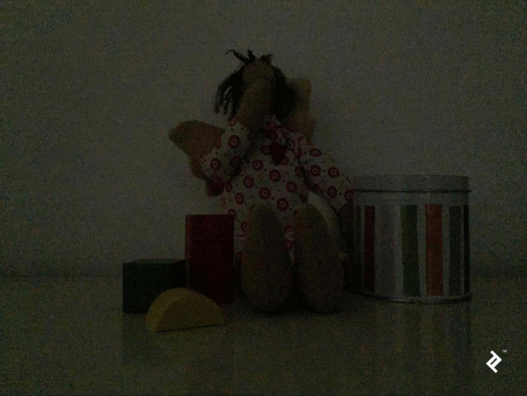
Attempting to enhance the contrast only worsens the image quality:

The root cause of this noise lies in the camera sensor, which struggles to accurately detect and measure light in low-light conditions. To compensate, the sensor increases its sensitivity, making it prone to detecting false signals or “noise.”

While noise is inherent in any imaging device, it becomes more prominent in low-light situations due to the weak signal. However, we can mitigate this issue even with hardware limitations.

The key lies in understanding that while the noise in multiple shots of a static scene is random, the actual signal remains constant. By averaging these images, we can effectively cancel out the random noise while preserving the true signal.

This principle is visually represented below:

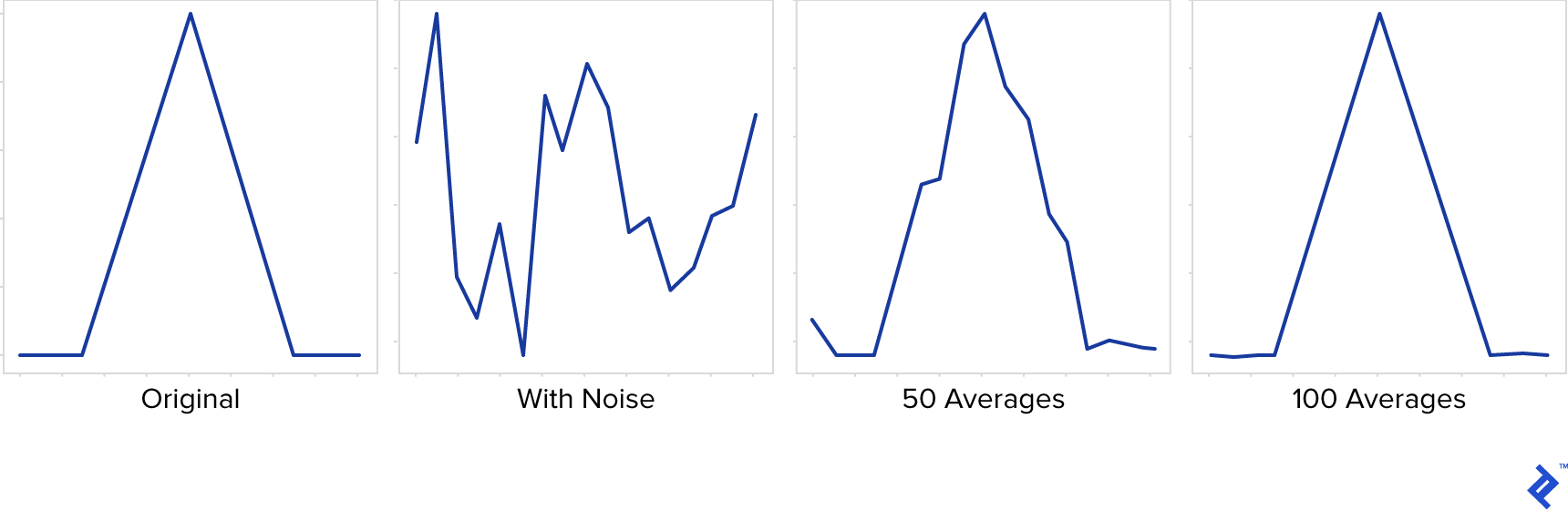
As evident, averaging multiple instances of the signal effectively reduces the noise, ultimately revealing the original signal.

Let’s apply this to images: Capture multiple shots of your subject at the highest exposure setting your camera allows. For optimal results, use a tripod and a manual camera app. The number of shots needed depends on various factors, but a range of 10 to 100 is often sufficient.

Once you have these raw format images, you can process them using Python. For this, we’ll utilize two libraries: NumPy (http://www.numpy.org/) and OpenCV (https://opencv.org/). NumPy facilitates efficient array computations, while OpenCV enables image file handling and offers advanced graphics processing capabilities.

 1
 2
 3
 4
 5
 6
 7
 8
 9
10
11
12
13
14
15
16
17
18
19
20
21
22
23
24
25
26
27

import os
import numpy as np
import cv2

folder = 'source_folder'

# We get all the image files from the source folder
files = list([os.path.join(folder, f) for f in os.listdir(folder)])

# We compute the average by adding up the images
# Start from an explicitly set as floating point, in order to force the
# conversion of the 8-bit values from the images, which would otherwise overflow
average = cv2.imread(files[0]).astype(np.float)
for file in files[1:]:
    image = cv2.imread(file)
    # NumPy adds two images element wise, so pixel by pixel / channel by channel
    average += image
 
# Divide by count (again each pixel/channel is divided)
average /= len(files)

# Normalize the image, to spread the pixel intensities across 0..255
# This will brighten the image without losing information
output = cv2.normalize(average, None, 0, 255, cv2.NORM_MINMAX)

# Save the output
cv2.imwrite('output.png', output)

The output, after auto-contrast adjustment, demonstrates significant noise reduction compared to the original image.

However, we still observe artifacts like the greenish frame and grid-like pattern, indicating a fixed pattern noise stemming from sensor inconsistencies.

This pattern arises from variations in the sensor’s response to light, leading to a visible pattern. Some patterns might be regular, likely related to the sensor material and its light interaction properties, while others, like the white pixel, could indicate defective sensor pixels with unusual light sensitivity.

To address this, we can employ a technique called dark frame subtraction. This involves capturing the pattern noise itself by photographing darkness. By averaging numerous dark frames captured at maximum exposure and ISO, we obtain an image representing the fixed pattern noise. This image can then be reused to correct future low-light shots.

Here’s a sample of the top-right portion of the pattern noise (contrast adjusted) from an iPhone 6:

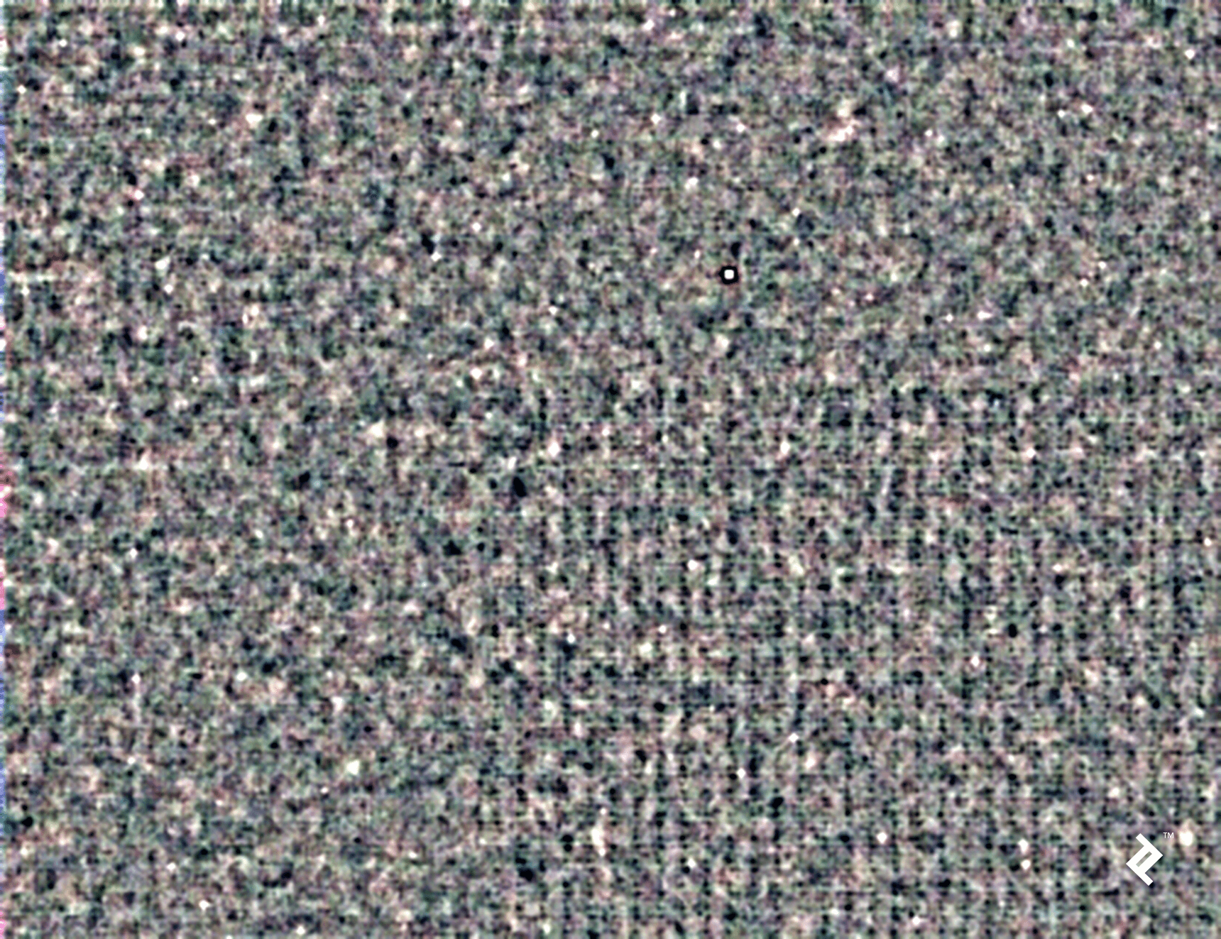
The grid-like texture and even a potentially stuck white pixel are visible.

By subtracting this dark frame noise (stored in the average_noise variable) from our image before normalization, we get:

1
2
3
4

average -= average_noise

output = cv2.normalize(average, None, 0, 255, cv2.NORM_MINMAX)
cv2.imwrite('output.png', output)

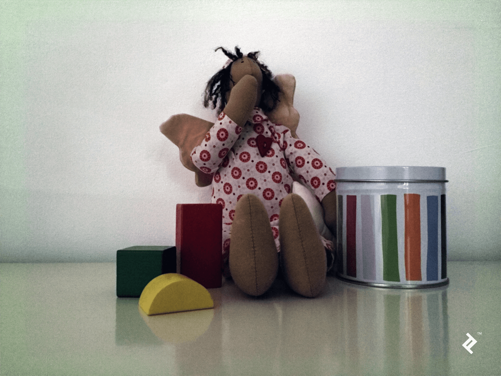
Leading to our final, improved image:

High Dynamic Range

Another constraint of smaller cameras, particularly mobile ones, is their limited dynamic range, restricting their ability to capture details across a wide range of light intensities.

In simpler terms, these cameras can only effectively capture a narrow band of light intensities. Details in areas that are too dark appear as pure black, while overly bright regions are rendered as pure white, resulting in a loss of detail.

While adjusting the exposure time can shift this capturable range, it often involves compromising details in other areas of the image. The following three images of the same scene illustrate this, each captured at a different exposure time: a short exposure (1/1000 sec), a medium exposure (1/50 sec), and a long exposure (1/4 sec).

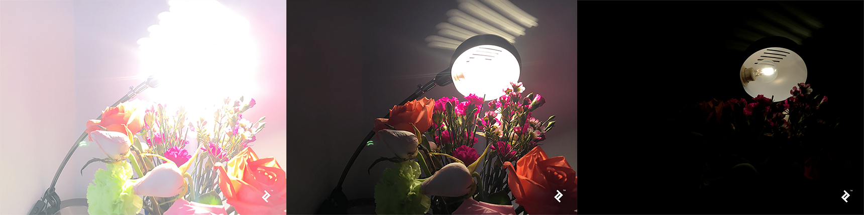
As evident, none of the images capture all the details comprehensively. The lamp’s filament is only visible in the first, while certain flower details are present in either the second or third image but not both.

Fortunately, we can overcome this limitation by leveraging multiple shots and Python code. Our approach is based on the work of Paul Debevec et al., detailed in their paper here.

The process begins with capturing multiple shots of the stationary scene at varying exposure times, ensuring the camera remains steady using a tripod. A manual camera app is also necessary to control exposure time and prevent automatic adjustments. The number of shots and the exposure time range depend on the scene’s intensity range, ensuring all essential details are captured in at least one shot.

Next, an algorithm reconstructs the camera’s response curve using the color information of the same pixels across different exposures. This establishes a mapping between a point’s actual brightness, exposure time, and its corresponding pixel value in the captured image. We will be using OpenCV’s implementation of Debevec’s method.

1
2
3
4
5
6
7
8
9

# Read all the files with OpenCV
files = ['1.jpg', '2.jpg', '3.jpg', '4.jpg', '5.jpg']
images = list([cv2.imread(f) for f in files])
# Compute the exposure times in seconds
exposures = np.float32([1. / t for t in [1000, 500, 100, 50, 10]])

# Compute the response curve
calibration = cv2.createCalibrateDebevec()
response = calibration.process(images, exposures)

The generated response curve typically resembles this:

The vertical axis represents the combined effect of scene brightness and exposure time, while the horizontal axis represents the corresponding pixel value (0 to 255 per channel).

This curve then enables us to reverse the process. Given a pixel value and its exposure time, we can calculate the actual brightness of each scene point. This brightness value, known as irradiance, represents the light energy falling on a unit of sensor area and is represented using floating-point numbers to accommodate a wider range of values, hence achieving high dynamic range. The generated irradiance map, or HDR image, can then be saved:

1
2
3
4
5
6

# Compute the HDR image
merge = cv2.createMergeDebevec()
hdr = merge.process(images, exposures, response)

# Save it to disk
cv2.imwrite('hdr_image.hdr', hdr)

Those fortunate enough to have HDR displays can visualize this image directly. However, given that HDR standards are still evolving, the display process might vary.

For those without HDR displays, we can still utilize this data, albeit with some adaptations for standard displays that require byte value (0-255) channels. This conversion, called tone-mapping, involves transforming the high-range floating-point irradiance map into a standard byte value image. Various techniques can help preserve details during this conversion. For instance, before compressing the floating-point range, we can enhance edges in the HDR image, helping retain these details in the final low dynamic range image.

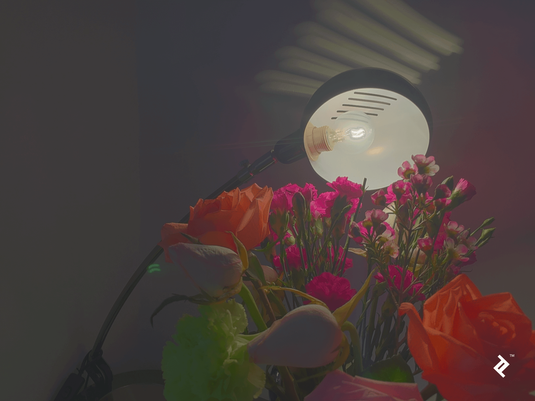
OpenCV offers several tone-mapping operators for this purpose, including Drago, Durand, Mantiuk, and Reinhardt. Below is an example demonstrating the Durand operator and its output.

1
2
3
4
5
6

durand = cv2.createTonemapDurand(gamma=2.5)
ldr = durand.process(hdr)

# Tonemap operators create floating point images with values in the 0..1 range
# This is why we multiply the image with 255 before saving
cv2.imwrite('durand_image.png', ldr * 255)

Python also allows for creating custom operators for greater control. Here’s the output from a custom operator that removes rarely occurring intensities before compressing the value range to 8 bits, followed by auto-contrast:

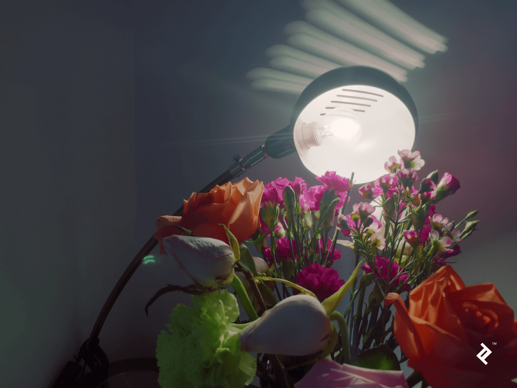
And here’s the code for this custom operator:

 1
 2
 3
 4
 5
 6
 7
 8
 9
10
11
12

def countTonemap(hdr, min_fraction=0.0005):
	counts, ranges = np.histogram(hdr, 256)
	min_count = min_fraction * hdr.size
	delta_range = ranges[1] - ranges[0]

	image = hdr.copy()
	for i in range(len(counts)):
    	if counts[i] < min_count:
        	image[image >= ranges[i + 1]] -= delta_range
        	ranges -= delta_range

	return cv2.normalize(image, None, 0, 1, cv2.NORM_MINMAX)

Conclusion

As demonstrated, Python, along with libraries like NumPy and OpenCV, allows us to push the boundaries of physical camera limitations and achieve superior image quality. Both examples showcase how combining multiple lower-quality shots can produce a better final result. Numerous other approaches can address specific problems and constraints.

While many camera phones incorporate built-in features for these enhancements, manually implementing them using code provides a deeper understanding and greater control over the process.

For those interested in exploring image processing on mobile devices, check out this OpenCV Tutorial: Real-time Object Detection Using MSER in iOS by Toptaler and elite OpenCV developer Altaibayar Tseveenbayar.