Have you ever flipped through an old photo album and found yourself smiling at memories you almost forgot? For me, it might be wearing a costume to sing “Barbie Girl” in a sixth-grade performance, holding my baby brother for the first time, or some other awkward, happy, or funny event. Some of those moments will only exist in the album. (I’m pretty sure my mom won’t be having any more kids, though I could ask.) On the other hand, these memories can also inspire future plans – maybe a reunion with my fellow Aqua impersonators!

You’re probably wondering what this has to do with anything by now. But the life of a PPC account is similar! There are ups and downs, and we often forget the good times. Reviewing your account’s past performance can help you make better decisions in the future. Plus, comparing your account to a high-performing month in the past can give you a good idea of where you are and where you can improve. At Hanapin, I use Excel. Using Excel to analyze past changes makes it easier to plan for the future. Try these easy steps and let Excel analyze your account for you.

Comparing Your PPC Account Month to Month

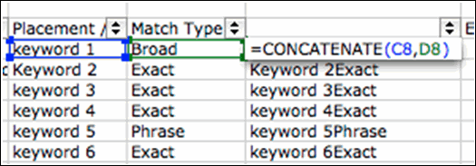
1. Get a keyword report for the month you want to look at. (If it’s not over yet, use last month’s, so you have enough data.) Include everything you want to compare. 2. Export the report. 3. Create the same report for the month you want to compare it to. I use the same month from the previous year to avoid seasonal variations, but you can use the best month of the past year. 4. Make sure both reports are in the same file – copy and paste the second month into a new tab. Name each sheet so you can tell them apart. 5. Make sure Excel can tell the difference between keywords with different match types. Since Excel can only refer to one cell at a time, put the keyword and its match type in the same cell. To do this, add a new column after ‘Match Type’ and combine the keyword and match type using the formula Concatenate=(Cell1, Cell2). You can add a space between the cells, but do it the same way in both sheets.

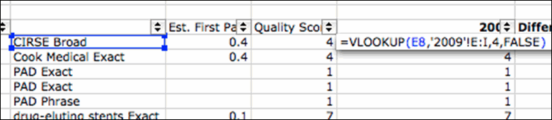
6. Now we’ll use a VLookup. This formula searches for your keyword in the second sheet and returns the corresponding data. We need a VLookup because the keywords won’t be in the same order on both sheets and it would take forever to do it manually! VLookups can be tricky if you don’t speak Excel – but they’re really easy once you’ve done one, so stick with me! We’ll break it down: a. In your most recent month’s sheet, add a column after each metric you want to compare – clicks, position, conversions, etc. b. In the first blank column, type =VLOOKUP( – then click the combined keyword/match type cell.

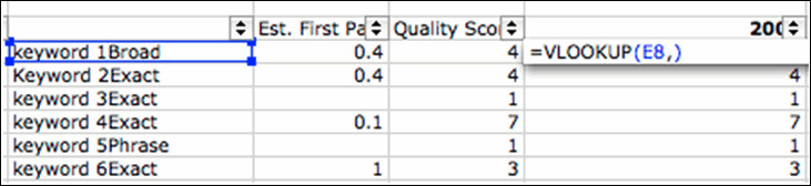
c. Add a comma after the cell number, then switch to the second sheet and select all the columns from the combined cell to the data you want to compare (in this example, it’s Quality Score).

d. Add another comma, then count the columns from your reference cell to the data you want. (Make sure you’re looking at the second sheet since the first sheet has those extra columns.) In this case, it is four. Type the number, another comma, and the word false. *You can’t look up anything to the left of your reference cell, so make sure the reference cells in both sheets are on the left side of any data you want to compare.

7. Repeat that for every metric you want to pull from the historical month and extend the formulas down. I recommend creating another column to see the difference between the two months – just subtract the past month’s data from the current month’s data. A negative difference generally isn’t good - it means your Quality Score, impressions, clicks, or conversions have gone down. (Unless you’re looking at ad position - in that case, a negative number means improvement.) 8. To avoid checking every single number, select each difference column while holding down control (command on a Mac). Then, click Conditional Formatting in the Format menu.

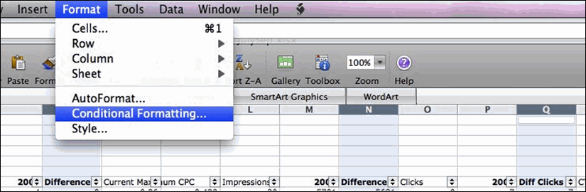
9. The Conditional Formatting box will pop up. Select ‘less than’ from the second drop-down menu and type 0 in the last box. Then click Format, choose a color under the Fill tab, and hit OK. Now, any negative differences will be highlighted.

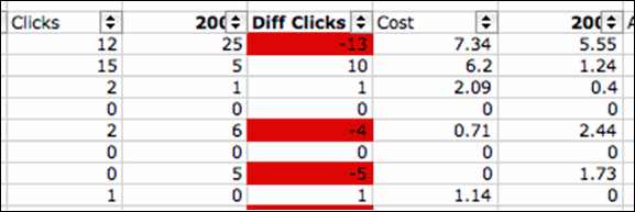
I like this approach because it highlights the source of the issue. If your clicks, conversions, and ad position have all dropped, you might need to increase your bids to show up higher in search results. If your ad position hasn’t changed but clicks have decreased, make sure your ads are relevant and targeted; if they don’t fit some of the keywords in their ad groups, you might need to write new ads or restructure your campaigns. These might seem obvious, but it’s easy for this kind of problem to slip by unnoticed in a busy account. I like to create these reports monthly, or at least every few months, to make sure the account is in top shape. You can use this for almost any comparison. Want an even deeper analysis? Apply conditional formatting to individual columns with more specific rules. For example, you could format your click difference column to turn orange for values between 0 and -200, and red for anything less than -200. This will give you a more detailed view of your data. Turns out Excel can be as much fun as a photo album! I hope this helps you as much as it’s helped me - give it a shot and let me know what you think! Amy Hoffman is a search marketing expert at Hanapin Marketing, and also writes for PPC Hero and SEO Boy.