I’ve been captivated by generative adversarial networks (GANs) ever since I discovered them. GANs are a category of neural networks capable of generating completely new data. By feeding them a small amount of random noise as input, they can create realistic images of anything from bedrooms to birds, depending on their training.
It’s universally acknowledged in the scientific community that we require more data. GANs present a potentially valuable solution by generating new data in situations where data is scarce. Data acquisition can often be a costly, time-intensive, and challenging endeavor. However, for this generated data to be truly useful, it needs to be sufficiently realistic so that any insights gleaned from it hold true for real-world data. Imagine training a cat to hunt using fake mice – those fake mice need to convincingly resemble real ones for the training to be effective.
Another perspective is that GANs uncover underlying patterns within data, enabling them to generate realistic representations. This capability proves particularly useful when these patterns remain hidden from human observation or elude extraction through other methods.
This article will guide you through the process of leveraging GANs for generating new data. To ensure practicality, we’ll utilize the credit card fraud detection dataset sourced from Kaggle.
During my experimentation, I used this dataset to determine if a GAN could create data realistic enough to aid in fraud detection. This dataset highlights the challenge of limited data: Out of 285,000 transactions, only 492 are fraudulent. 492 instances of fraud constitute a limited dataset for training, especially in machine learning, where larger datasets are generally preferred. While my experiment didn’t yield extraordinary results, the insights gained about GANs during the process are valuable and worth sharing.
Before You Start
Before diving into the world of GANs, if you wish to refresh your machine learning or deep learning knowledge, consider exploring these relevant blog posts:
- An Introduction to Machine Learning Theory and Its Application: A Visual Tutorial with Examples
- A Deep Learning Tutorial: From Perceptrons to Deep Networks
Why GANs?
Generative adversarial networks (GANs) have emerged as a neural network architecture that has demonstrated significant advantages over earlier generative approaches, such as variational auto-encoders or restricted Boltzmann machines. GANs have exhibited capabilities like generating more realistic images (e.g., DCGAN), facilitating style transfer between images (refer to here and here), producing images from textual descriptions (StackGAN), and learning effectively from smaller datasets through semi-supervised learning. These accomplishments have garnered substantial interest in both academic and commercial domains.
Yann LeCunn, the Director of AI Research at Facebook, has even hailed them as the most exciting development in machine learning of the last decade.
The Basics
Consider your own learning process. You attempt something, receive feedback, adjust your approach, and try again.
Feedback can take various forms – criticism, discomfort, or even rewards. It can stem from your own evaluation of your performance. Frequently, the most valuable feedback comes from another individual, as it goes beyond numerical scores to provide insightful analysis of your task execution.
When a computer undergoes training for a task, humans typically provide feedback through parameter adjustments or algorithm modifications. This approach works well for clearly defined tasks like multiplication. Conveying the computer’s errors in such cases is straightforward and precise.
However, providing feedback becomes more challenging with complex tasks like generating a dog image. Assessing whether the image is blurry, resembles a cat more, or if it’s even remotely recognizable becomes subjective. While complex statistics can be employed, encapsulating all the nuances that contribute to an image’s realism remains difficult.
Humans can offer estimations based on our extensive experience with visual input, but our evaluations can be inherently subjective and relatively slow. An alternative is to train a neural network to distinguish between real and generated images.
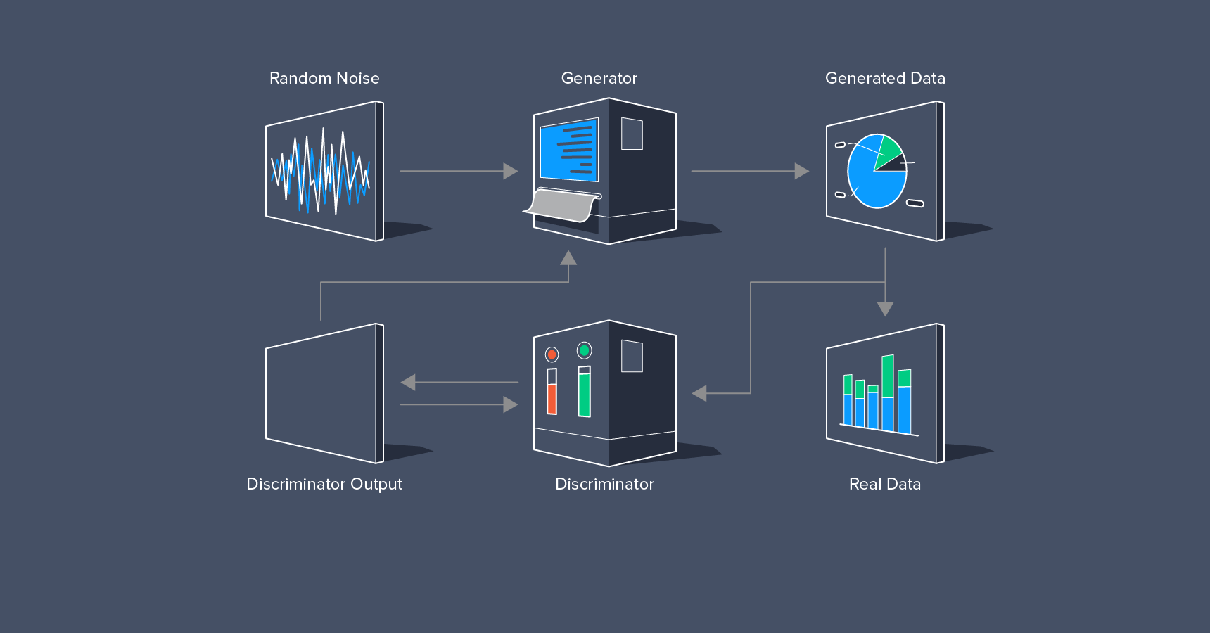
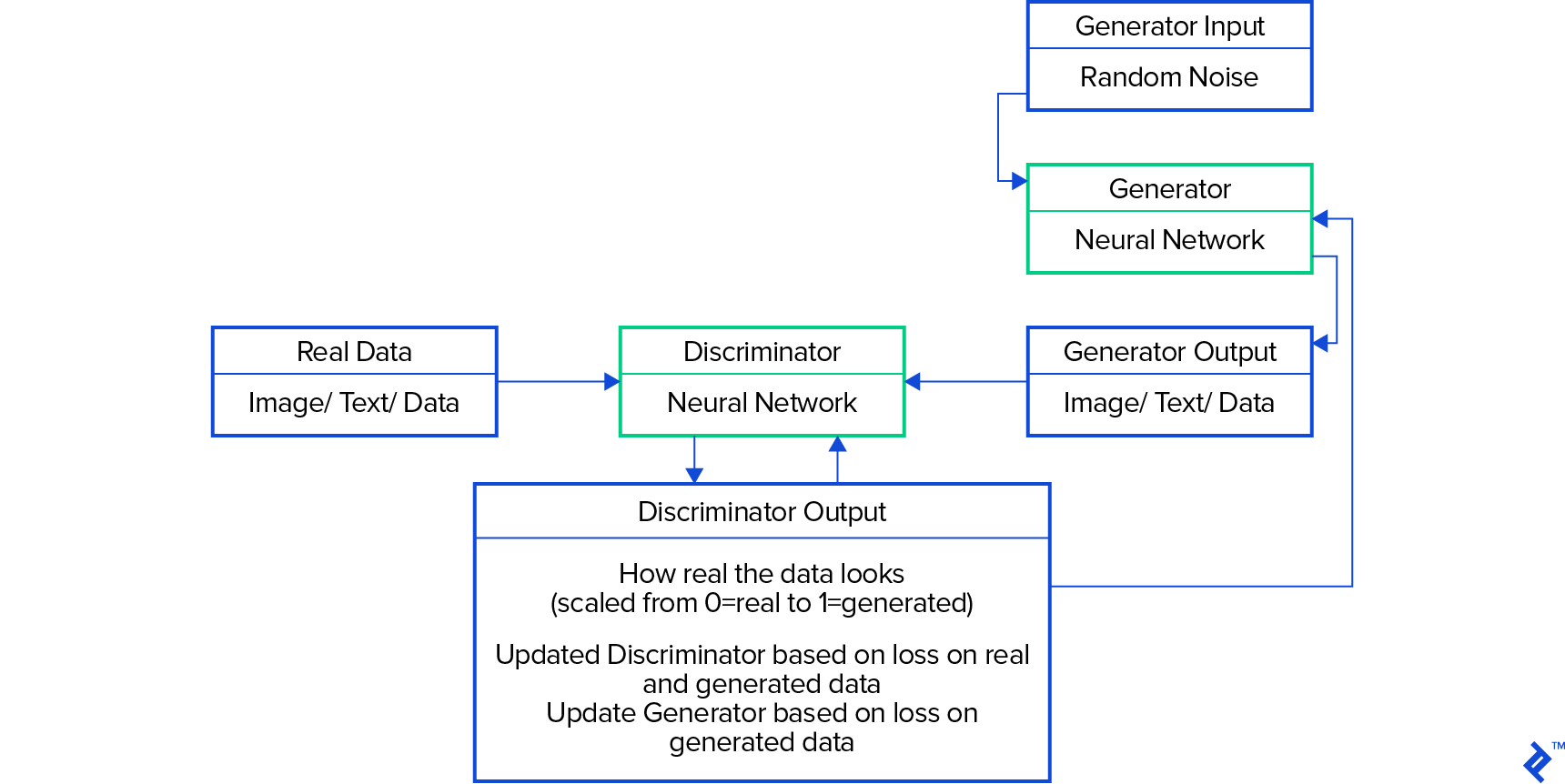
By enabling the image generator (also a neural network) and the discriminator to learn from each other iteratively, both improve over time. These two networks, engaged in this game, constitute a generative adversarial network.
You can hear a talk by Ian Goodfellow, the inventor of GANs, where he recounts how an argument at a bar on this subject sparked a night of intense coding that birthed the first GAN. Notably, he acknowledges the bar in his paper. Further insights into GANs can be gained from Ian Goodfellow’s blog on the topic.
Working with GANs presents several hurdles. Training even a single neural network can be challenging due to the multitude of decisions involved: network architecture, activation functions, optimization methods, learning rates, and dropout rates, to name a few.
GANs double these choices and introduce additional complexities. Both the generator and the discriminator might lose previously learned techniques during training. This can trap the networks in a cycle of stable yet suboptimal solutions. One network might overpower the other, hindering further learning. Alternatively, the generator might explore only a limited portion of the solution space, just enough to find plausible solutions—a phenomenon known as mode collapse.
Mode collapse occurs when the generator masters only a small subset of potential realistic modes. For instance, if tasked with generating dog images, the generator might only learn to create small brown dogs, missing other possibilities like different sizes or colors.
Numerous strategies combat this issue, including batch normalization, incorporating labels into the training data, or modifying the discriminator’s evaluation of generated data.
Adding labels to categorize data has been observed to consistently enhance GAN performance. Generating images of specific pet categories like cats, dogs, fish, and ferrets is considered more manageable than generating images of pets in general.
Perhaps the most significant advancements in GAN development lie in altering how the discriminator assesses data, so let’s delve into that aspect.
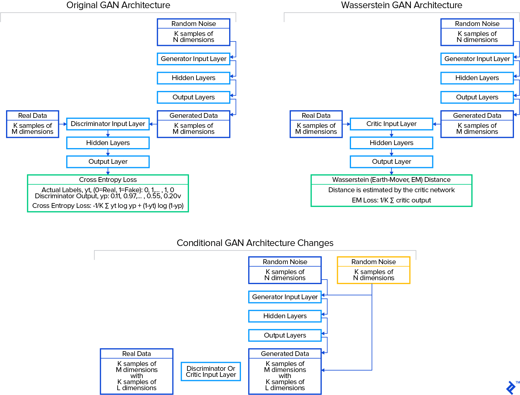
In the original 2014 GAN formulation by Goodfellow et al., the discriminator estimates the likelihood of an image being real or generated. Provided a mix of real and generated images, it assigns a probability to each. The discrepancy between the discriminator’s output and the actual labels is then measured using cross-entropy loss. This loss is analogous to the Jensen-Shannon distance metric, which Arjovsky et al. demonstrated in early 2017 could be unreliable, sometimes failing to provide a useful learning signal. They proposed the Wasserstein distance metric (also called earth mover or EM distance) as a more robust alternative.
Cross-entropy loss quantifies the discriminator’s accuracy in distinguishing real from generated images. Conversely, the Wasserstein metric examines the distribution of each variable (e.g., the color of each pixel) in both real and generated images, determining the disparity between these distributions. It conceptually measures the effort (mass times distance) required to reshape the generated distribution to match the real one, hence the name “earth mover distance.” Since the Wasserstein metric doesn’t classify images as real or fake but instead critiques the generated images’ deviation from real ones, the “discriminator” network is termed the “critic” network in the Wasserstein architecture.
For a slightly more comprehensive understanding of GANs, we’ll explore four architectures in this article:
- GAN: The original (“vanilla”) GAN
- CGAN: A conditional variant of the original GAN that utilizes class labels
- WGAN: The Wasserstein GAN (with gradient penalty)
- WCGAN: A conditional variant of the Wasserstein GAN
But first, let’s take a quick look at our dataset.
A Look at Credit Card Fraud Data
Our focus will be on the credit card fraud detection dataset from Kaggle.
This dataset comprises approximately 285,000 transactions, with only 492 being fraudulent. The data encompasses 31 features: “time,” “amount,” “class,” and 28 anonymized features. The “class” feature labels a transaction as fraudulent (1) or normal (0). All features are numeric and continuous, except the label. The dataset is complete, with no missing values. It’s already well-structured, requiring minimal cleaning, primarily adjusting feature means to zero and standard deviations to one. My cleaning process is detailed in the notebook here. For now, I’ll present the end result:
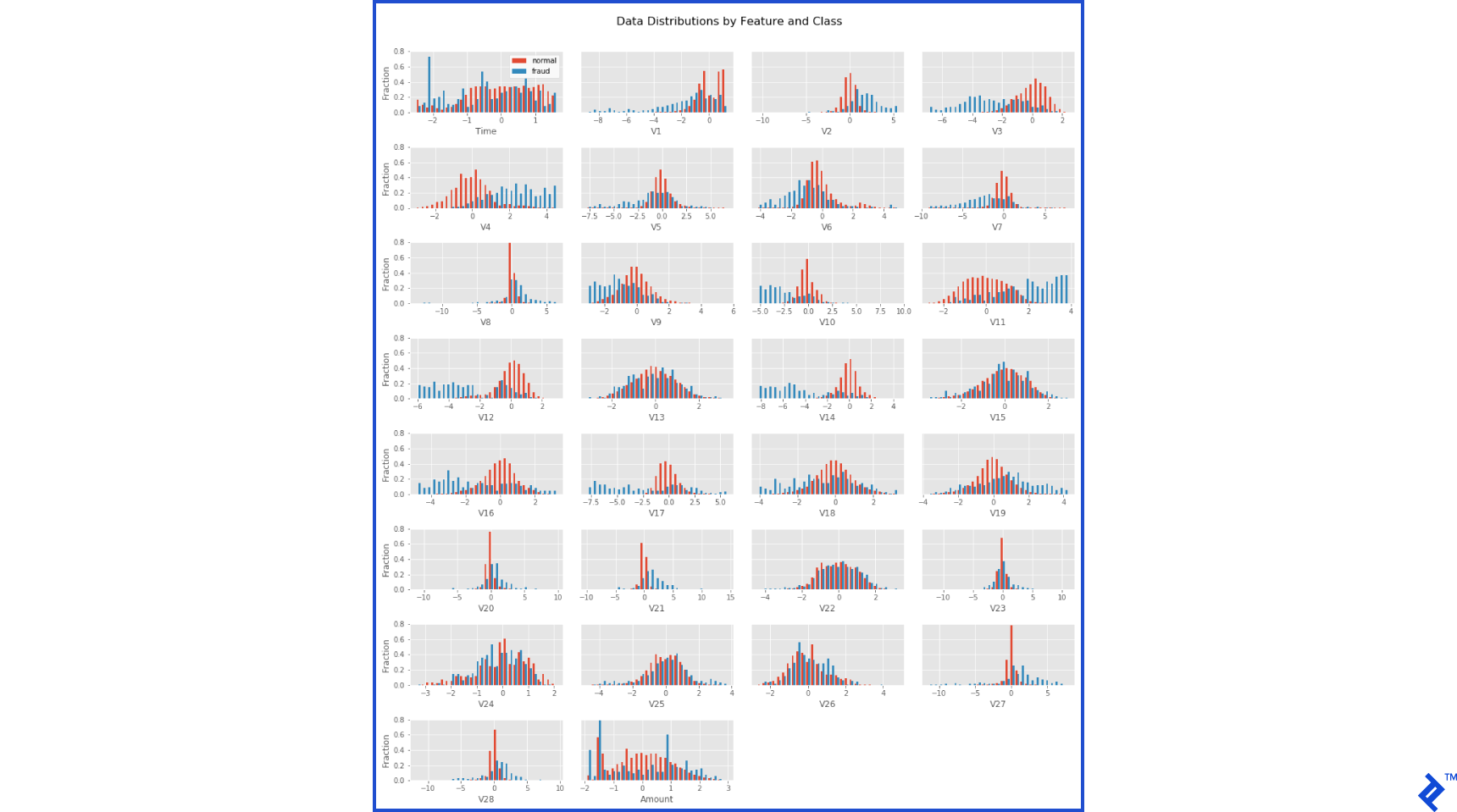
Distinguishing between normal and fraudulent transactions is fairly straightforward from these distributions, although considerable overlap exists. To pinpoint the most effective features for fraud detection, we can employ one of the faster and more powerful machine learning algorithms, xgboost – a gradient-boosted decision tree algorithm. Training on 70% of the dataset and testing on the remaining 30%, we allow the algorithm to run until it no longer improves recall (the fraction of fraud samples detected) on the test set. This achieves a 76% recall on the test set, indicating room for improvement. Notably, it achieves a precision of 94%, meaning only 6% of predicted fraud cases were actually normal. This analysis also ranks features by their fraud detection utility. These prominent features will later aid in result visualization.
Again, having more fraud data could potentially enhance detection rates, leading to higher recall. Our next step involves using GANs to generate new, realistic fraud data to improve actual fraud detection.
Generating New Credit Card Data with GANs
To apply different GAN architectures to this dataset, I’ll use GAN-Sandbox. This resource provides implementations of popular GAN architectures in Python using the Keras library with a TensorFlow backend. All results are available in a Jupyter notebook here. For ease of setup, the Kaggle/Python Docker image includes all necessary libraries.
The examples in GAN-Sandbox are designed for image processing. The generator produces a 2D image with three color channels per pixel, which the discriminator/critic evaluates. Convolutional layers within the networks exploit the spatial structure inherent in image data. Each neuron in a convolutional layer processes a small, localized input region (e.g., adjacent pixels), facilitating the learning of spatial relationships. However, our credit card dataset lacks such spatial structure. To address this, I’ve replaced the convolutional networks with densely connected layers. Neurons in these layers connect to all inputs and outputs, enabling the network to learn its own feature relationships. This setup will be consistent across all architectures.
The first GAN evaluated pits the generator against the discriminator, utilizing the discriminator’s cross-entropy loss for training. This is the original “vanilla” GAN. The second, a conditional GAN (CGAN), incorporates class labels. This GAN includes an additional variable in the data—the class label. The third, a Wasserstein GAN (WGAN), employs the Wasserstein distance metric for training. Finally, the last one, a WCGAN, uses both class labels and the Wasserstein distance metric.
Training the GANs will involve using a dataset consisting of all 492 fraudulent transactions. To facilitate the conditional GAN architectures, we’ll add classes to this fraud dataset. After exploring various clustering methods in the notebook, I opted for KMeans classification to categorize the fraud data into two classes.
Each GAN will undergo 5000 training rounds, with periodic result examinations. Figure 4 illustrates the actual and generated fraud data from different GAN architectures as training progresses. The actual fraud data, divided into two KMeans classes, is plotted along the two dimensions that best differentiate these classes (features V10 and V17 from PCA-transformed features). The non-conditional GAN and WGAN generate output belonging to a single class. The conditional architectures, CGAN and WCGAN, display generated data separated by class. At step 0, all generated data points resemble generated data shows due to the random input provided to the generators.
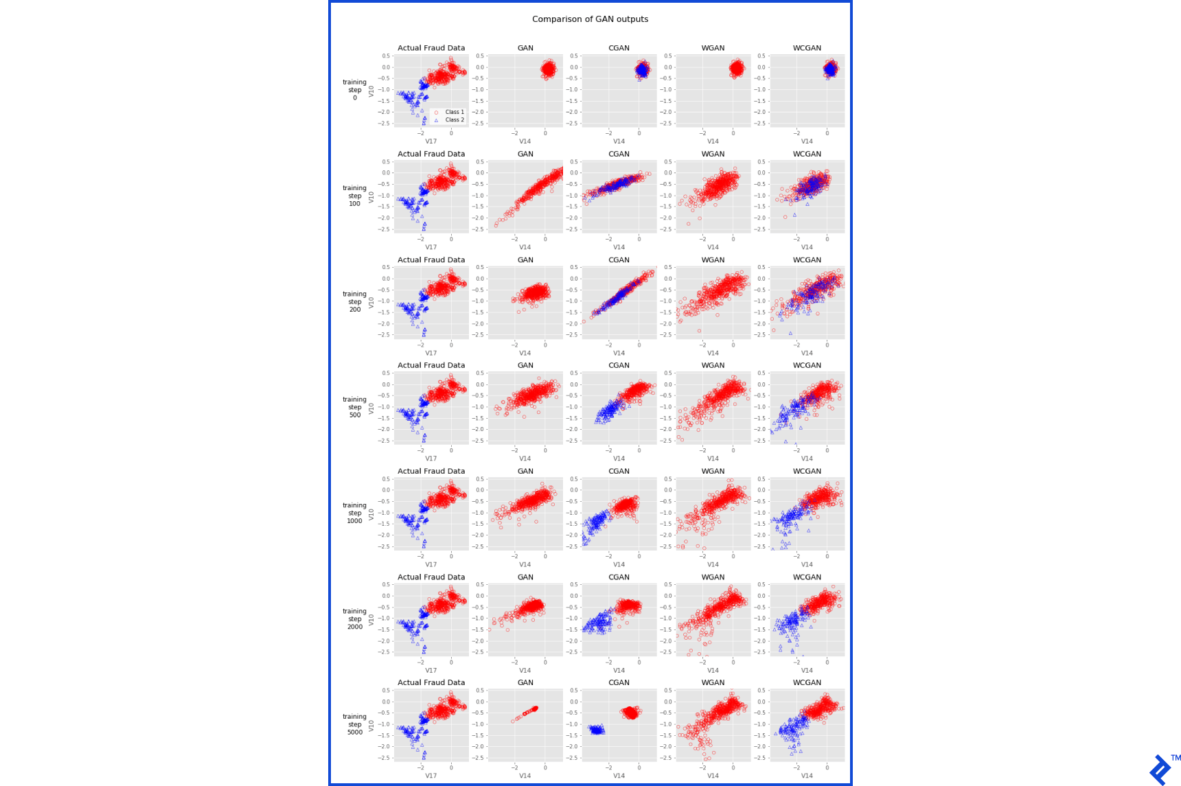
The original GAN architecture initially learns the shape and range of the actual data, but eventually collapses to a narrow distribution—an example of mode collapse. The generator has discovered a small data region that the discriminator struggles to classify as fake. The CGAN performs slightly better, spreading out and approaching the distributions of each fraud class. However, mode collapse eventually sets in, as evident at step 5000.
Unlike the GAN and CGAN, the WGAN does not exhibit mode collapse. Even without class information, it starts to approximate the non-normal distribution of the actual fraud data. The WCGAN demonstrates similar behavior, effectively generating distinct data classes.
To assess the realism of the generated data, we’ll utilize the same xgboost algorithm employed earlier for fraud detection. This algorithm is fast, powerful, and requires minimal tuning. We’ll train the xgboost classifier using half of the actual fraud data (246 samples) and an equal number of GAN-generated examples. Subsequently, it will be tested using the remaining half of the actual fraud data and a different set of 246 GAN-generated examples. This orthogonal approach provides an indication of the generator’s ability to produce realistic data. Ideally, with perfectly realistic generated data, the xgboost algorithm should achieve an accuracy of 0.50 (50%)—equivalent to random guessing.
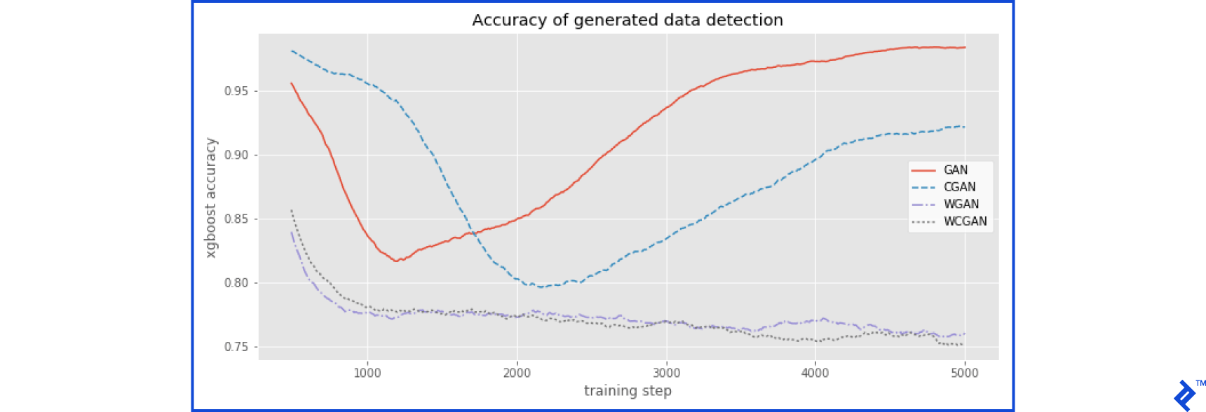
Observations indicate an initial decrease in the see the xgboost accuracy on data generated by the GAN, followed by an increase after training step 1000 as mode collapse sets in. The CGAN architecture achieves slightly more realistic data after 2000 steps, but eventually succumbs to mode collapse as well. The WGAN and WCGAN architectures generate more realistic data more rapidly and continue to learn throughout training. The WCGAN doesn’t appear significantly better than the WGAN, suggesting that these created classes might not be beneficial for Wasserstein GAN architectures.
For a deeper dive into the WGAN architecture, refer to here and here.
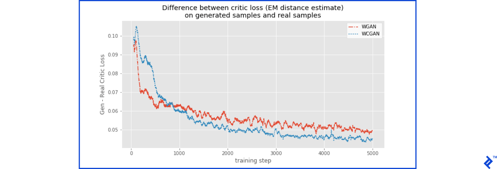
The critic network in the WGAN and WCGAN architectures learns to calculate the Wasserstein (Earth-mover, EM) distance between a given dataset and the actual fraud data. Ideally, it should measure a distance close to zero for actual fraud data. However, the critic is still learning this calculation. As long as it consistently assigns a larger distance to generated data compared to real data, the network can improve. By monitoring the difference in Wasserstein distances between generated and real data during training, we can identify plateaus that indicate potential training saturation. Figure 6 suggests that further improvement appears to be further improvement for both WGAN and WCGAN on this dataset.
What Did We Learn?
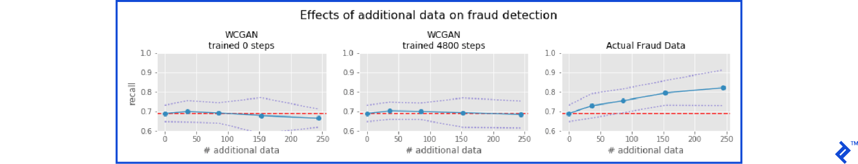
Now comes the test of whether the generated fraud data is realistic enough to aid in detecting actual fraud. We’ll select the trained generator that achieved the lowest accuracy score for data generation. The basic training set will consist of 70% of the non-fraud data (199,020 cases) and 100 cases of fraud data (approximately 20% of the fraud data). We’ll then experiment by augmenting this training set with varying amounts of real or generated fraud data, up to 344 cases (70% of the fraud data). The test set will comprise the remaining 30% of non-fraud cases (85,295 cases) and 148 fraud cases. To assess the effectiveness of generated data, we’ll compare using data from an untrained GAN, the best-trained GAN, and random noise. Based on our tests, the WCGAN at training step 4800 emerged as the most effective architecture, achieving an xgboost accuracy of 70% (recall that 50% represents random guessing). Therefore, we’ll utilize this architecture for generating new fraud data.
Figure 7 reveals that recall (the proportion of actual fraud samples correctly identified in the test set) does not improve with increasing amounts of generated fraud data used for training. The xgboost classifier effectively retains the information learned from the 100 real fraud cases and remains unaffected by the additional generated data, even when distinguishing them from a vast number of normal cases. Unsurprisingly, generated data from the untrained WCGAN has no discernible impact. However, even the data from the trained WCGAN fails to improve recall. This suggests that the generated data lacks sufficient realism. Figure 7 also shows that incorporating actual fraud data into the training set significantly boosts recall. If the WCGAN had simply memorized the training examples without generating novel variations, we would have observed higher recall rates as we see with the real data.
To Infinity and Beyond
Despite our inability to generate credit card fraud data realistic enough to enhance actual fraud detection, we’ve merely scratched the surface of these methods. Potential improvements include extending training durations, utilizing larger networks, and fine-tuning parameters for the explored architectures. The observed trends in xgboost accuracy and discriminator loss suggest that the WGAN and WCGAN architectures would benefit from further training. Revisiting data cleaning procedures, engineering new variables, or reevaluating the handling of feature skewness are other avenues for exploration. Exploring alternative fraud data classification schemes could also prove beneficial.
Experimenting with different GAN architectures is another possibility. The DRAGAN has demonstrated theoretical and empirical advantages over Wasserstein GANs in terms of training speed and stability. Integrating methods that leverage semi-supervised learning, which have shown potential in learning from limited datasets (see “Improved Techniques for Training GANs”), could be explored. Additionally, we could investigate architectures that yield human-interpretable models, potentially enhancing our understanding of the underlying data structure (see InfoGAN).
Staying abreast of emerging developments in the field is crucial, and equally important is the pursuit of our own innovations within this rapidly evolving domain.
The complete code for this article is available in this GitHub repository.