In the rapidly evolving landscape of technology, fields like machine learning, computer vision, API development, and UI design are experiencing remarkable advancements. While the former two delve into the complexities of mathematics and science, the latter two emphasize algorithmic thinking and crafting adaptable architectures. Despite their differences, these domains converge seamlessly in the realm of image processing applications.

This article aims to illustrate how these four areas can be harmoniously integrated to create an image processing application, specifically a straightforward digit recognizer. The simplicity of our chosen application will enable us to grasp the overarching concepts without getting bogged down in intricate details.

We will leverage user-friendly and widely adopted technologies for this endeavor. Python will serve as the backbone for the machine learning aspect, while the interactive front-end will be built using the ubiquitous JavaScript library, React.

Leveraging Machine Learning for Digit Recognition

At the heart of our application lies an algorithm tasked with deciphering handwritten digits, a task we will entrust to the capabilities of machine learning. This form of artificial intelligence empowers systems to learn autonomously from provided data. Essentially, machine learning is about identifying patterns or correlations within data and extrapolating those patterns to make predictions.

Our image recognition process can be broken down into three key stages:

• Procuring images of handwritten digits for training purposes
• Training the system to recognize digits based on the provided training data
• Evaluating the system’s performance using new, unseen data

Setting Up the Environment

To work with machine learning in Python, we require a virtual environment, a practical solution that handles all the necessary Python packages, sparing us from tedious configuration.

Let’s proceed with the installation using the following terminal commands:

1
2

python3 -m venv virtualenv
source virtualenv/bin/activate

Training the Model

Before diving into code, selecting a suitable “teacher” for our machine learning model is crucial. Data scientists often experiment with various models to pinpoint the most effective one. For our purposes, we’ll bypass complex models requiring extensive expertise and opt for the k-nearest neighbors algorithm.

This algorithm excels at categorizing data points on a plane based on specific features. To illustrate, consider the following image:

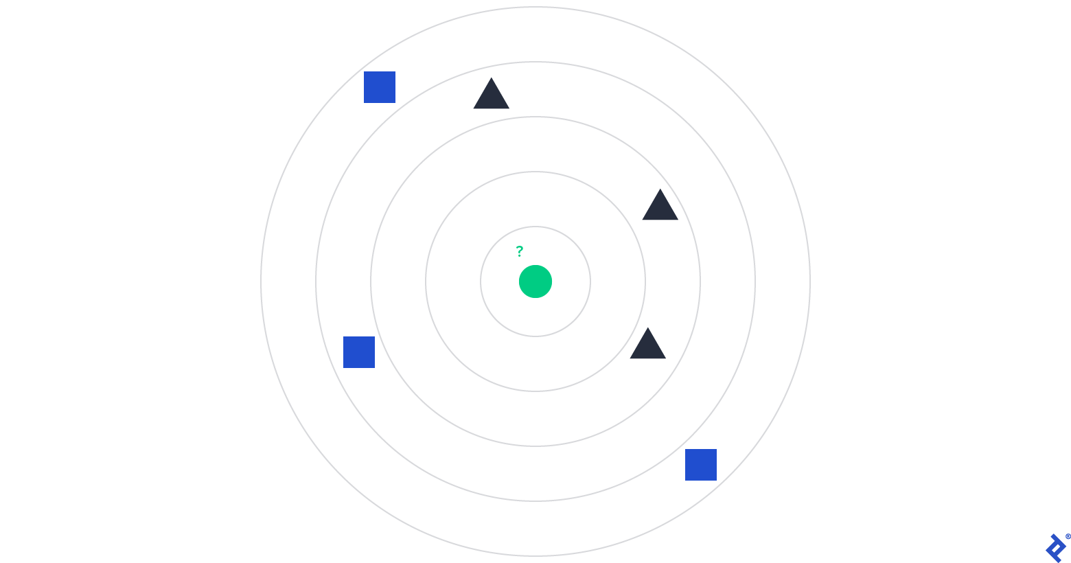
To determine the type of the Green Dot, we examine the types of its k nearest neighbors, where k is a predefined parameter. Referring to the image, if k is set to 1, 2, 3, or 4, the algorithm would classify the Green Dot as a Black Triangle, as most of its closest neighbors fall into that category. However, if we increase k to 5, the majority shifts to Blue Squares, leading to a classification of Blue Square.

To construct our machine learning model, we need several dependencies:

• sklearn.neighbors.KNeighborsClassifier: This is our chosen classifier.
• sklearn.model_selection.train_test_split: This function helps us divide our data into training and testing sets.
• sklearn.model_selection.cross_val_score: This function evaluates the model’s accuracy, with higher values indicating better performance.
• sklearn.metrics.classification_report: This function provides a detailed statistical report of the model’s predictions.
• sklearn.datasets: This package offers access to datasets, including the MNIST dataset we’ll be using.
• numpy: A cornerstone in scientific computing, NumPy enables efficient manipulation of multidimensional arrays in Python.
• matplotlib.pyplot: This package allows us to visualize data.

Let’s start by installing and importing these dependencies:

1
2
3
4
5
6
7

pip install sklearn numpy matplotlib scipy

from sklearn.datasets import load_digits
from sklearn.neighbors import KNeighborsClassifier
from sklearn.model_selection import train_test_split, cross_val_score
import numpy as np
import matplotlib.pyplot as plt 

Next, we load the MNIST Database, a widely used dataset of handwritten digit images frequently employed by those new to machine learning:

1

digits = load_digits()

With our data loaded, we split it into training and testing sets. We’ll allocate 75% for training our model and reserve the remaining 25% for evaluating its accuracy:

1
2
3

(X_train, X_test, y_train, y_test) = train_test_split(
    digits.data, digits.target, test_size=0.25, random_state=42
)

Now, we need to determine the optimal k value for our model to enhance its predictive accuracy. Let’s explore why experimenting with different k values is essential:

 1
 2
 3
 4
 5
 6
 7
 8
 9
10
11
12

ks = np.arange(2, 10)
scores = []
for k in ks:
    model = KNeighborsClassifier(n_neighbors=k)
    score = cross_val_score(model, X_train, y_train, cv=5)
    score.mean()
    scores.append(score.mean())

plt.plot(scores, ks)
plt.xlabel('accuracy')
plt.ylabel('k')
plt.show()

Executing this code generates a plot illustrating the algorithm’s accuracy across various k values.

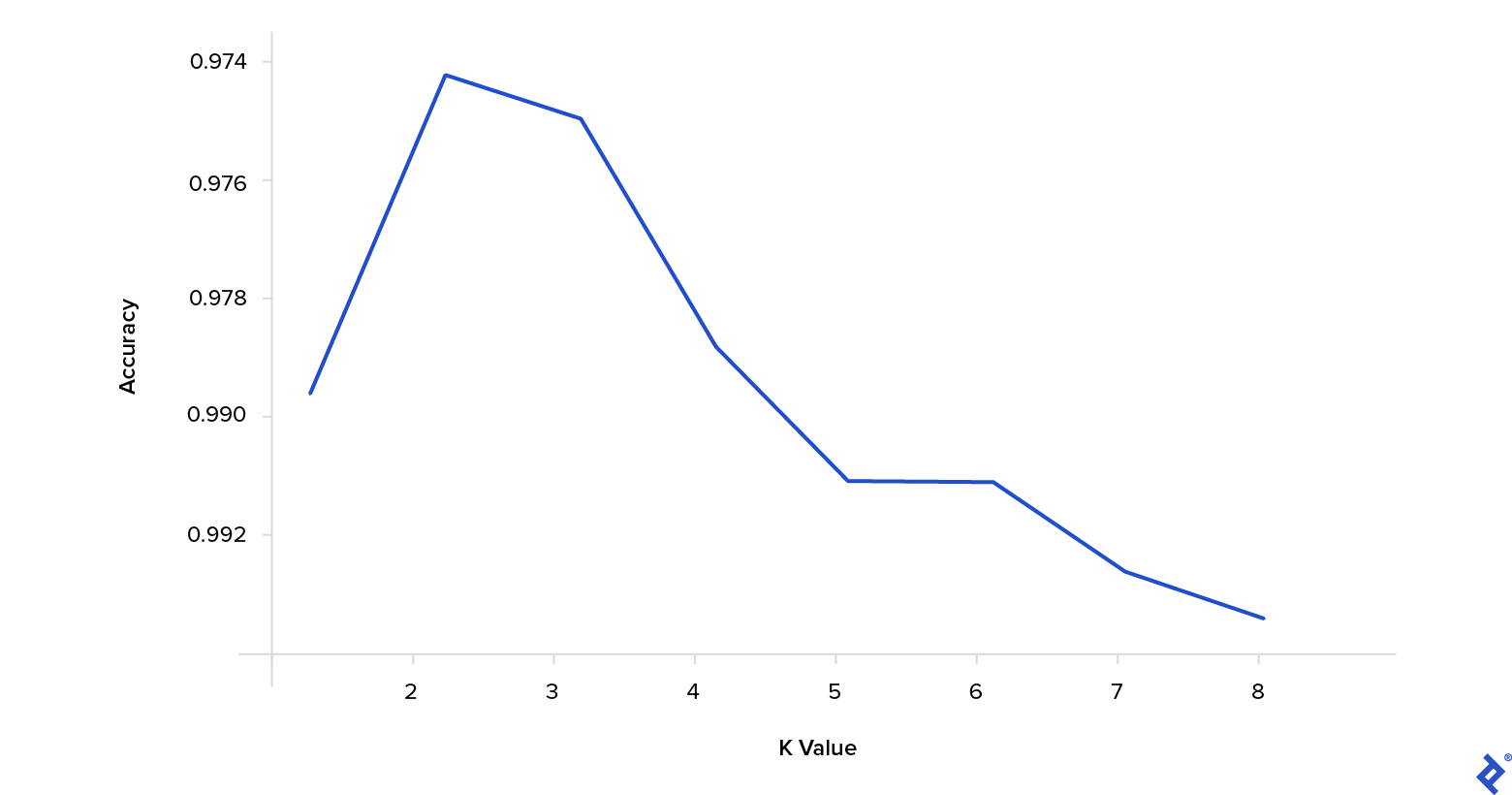
As evident from the plot, a k value of 3 yields the highest accuracy for our chosen model and dataset.

Constructing an API with Flask

Having built the core functionality—an algorithm for predicting digits from images—our next task is to encapsulate it within an API. For this, we’ll utilize the popular and lightweight Flask web framework.

Let’s begin by installing Flask and the necessary image processing dependencies within our virtual environment:

1

pip install Flask Pillow scikit-image

With the installation complete, we create the main entry point file for our application:

1

touch app.py

This file will contain the following code:

 1
 2
 3
 4
 5
 6
 7
 8
 9
10
11
12
13
14
15
16
17
18
19
20
21
22

import os

from flask import Flask
from views import PredictDigitView, IndexView

app = Flask(__name__)

app.add_url_rule(
    '/api/predict',
    view_func=PredictDigitView.as_view('predict_digit'),
    methods=['POST']
)

app.add_url_rule(
    '/',
    view_func=IndexView.as_view('index'),
    methods=['GET']
)

if __name__ == 'main':
    port = int(os.environ.get("PORT", 5000))
    app.run(host='0.0.0.0', port=port)

At this stage, we’ll encounter errors indicating that PredictDigitView and IndexView are not defined. To resolve this, we create a file to initialize these views:

 1
 2
 3
 4
 5
 6
 7
 8
 9
10
11
12
13
14
15
16
17
18
19
20

from flask import render_template, request, Response
from flask.views import MethodView, View

from flask.views import View

from repo import ClassifierRepo
from services import PredictDigitService
from settings import CLASSIFIER_STORAGE

class IndexView(View):
    def dispatch_request(self):
        return render_template('index.html')

class PredictDigitView(MethodView):
    def post(self):
        repo = ClassifierRepo(CLASSIFIER_STORAGE)
        service = PredictDigitService(repo)
        image_data_uri = request.json['image']
        prediction = service.handle(image_data_uri)
        return Response(str(prediction).encode(), status=200)

This will lead to further errors related to an unresolved import. Our Views package depends on three missing files:

• Settings
• Repo
• Service

Let’s implement each of these.

The Settings module will house configuration settings and constants, including the path to our serialized classifier. This raises a valid question: Why save the classifier?

Storing the trained classifier is a straightforward optimization technique. Instead of retraining the model with each request, we can load the pre-trained version, enabling our app to respond rapidly.

1
2
3
4

import os

BASE_DIR = os.getcwd()
CLASSIFIER_STORAGE = os.path.join(BASE_DIR, 'storage/classifier.txt')

Next, the Repo class provides mechanisms to retrieve and update the trained classifier using Python’s built-in pickle module:

 1
 2
 3
 4
 5
 6
 7
 8
 9
10
11
12
13
14
15
16
17
18
19
20

import pickle

class ClassifierRepo:
    def __init__(self, storage):
        self.storage = storage

    def get(self):
        with open(self.storage, 'wb') as out:
            try:
                classifier_str = out.read()
                if classifier_str != '':
                    return pickle.loads(classifier_str)
                else:
                    return None
            except Exception:
                return None

    def update(self, classifier):
        with open(self.storage, 'wb') as in_:
            pickle.dump(classifier, in_)

Our API is nearing completion, with only the Service module left to implement. This module handles the following:

• Loading the trained classifier from storage
• Transforming images received from the UI into a format compatible with the classifier
• Performing the prediction using the formatted image
• Returning the prediction result

Let’s translate this logic into code:

 1
 2
 3
 4
 5
 6
 7
 8
 9
10
11
12
13
14
15
16
17
18
19
20
21
22
23
24
25

from sklearn.datasets import load_digits

from classifier import ClassifierFactory
from image_processing import process_image

class PredictDigitService:
    def __init__(self, repo):
        self.repo = repo

    def handle(self, image_data_uri):
        classifier = self.repo.get()
        if classifier is None:
            digits = load_digits()
            classifier = ClassifierFactory.create_with_fit(
                digits.data,
                digits.target
            )
            self.repo.update(classifier)
        
        x = process_image(image_data_uri)
        if x is None:
            return 0

        prediction = classifier.predict(x)[0]
        return prediction

Notice that PredictDigitService relies on two dependencies: ClassifierFactory and process_image.

We’ll start by defining a class responsible for creating and training our model:

1
2
3
4
5
6
7
8
9

from sklearn.model_selection import train_test_split
from sklearn.neighbors import KNeighborsClassifier

class ClassifierFactory:
    @staticmethod
    def create_with_fit(data, target):
        model = KNeighborsClassifier(n_neighbors=3)
        model.fit(data, target)
        return model

With our API ready for action, let’s move on to the image processing stage.

Image Processing

Image processing encompasses a range of techniques applied to images to enhance them or extract meaningful information. In our case, we need to seamlessly convert user-drawn images into a format suitable for our machine learning model.

Let’s import some helper functions to achieve this:

1
2
3
4
5

import numpy as np
from skimage import exposure
import base64
from PIL import Image, ImageOps, ImageChops
from io import BytesIO

We can break down this image transformation process into six steps:

1. Replacing Transparent Backgrounds with Color

 1
 2
 3
 4
 5
 6
 7
 8
 9
10
11
12
13
14

def replace_transparent_background(image):
    image_arr = np.array(image)

    if len(image_arr.shape) == 2:
        return image

    alpha1 = 0
    r2, g2, b2, alpha2 = 255, 255, 255, 255

    red, green, blue, alpha = image_arr[:, :, 0], image_arr[:, :, 1], image_arr[:, :, 2], image_arr[:, :, 3]
    mask = (alpha == alpha1)
    image_arr[:, :, :4][mask] = [r2, g2, b2, alpha2]

    return Image.fromarray(image_arr)

2. Trimming Excess Borders

1
2
3
4
5
6
7
8
9

def trim_borders(image):
    bg = Image.new(image.mode, image.size, image.getpixel((0,0)))
    diff = ImageChops.difference(image, bg)
    diff = ImageChops.add(diff, diff, 2.0, -100)
    bbox = diff.getbbox()
    if bbox:
        return image.crop(bbox)
    
    return image

3. Adding Uniform Borders

1
2

def pad_image(image):
    return ImageOps.expand(image, border=30, fill='#fff')

4. Converting to Grayscale

1
2

def to_grayscale(image):
    return image.convert('L')

5. Inverting Colors

1
2

def invert_colors(image):
    return ImageOps.invert(image)

6. Resizing to 8x8 Format

1
2

def resize_image(image):
    return image.resize((8, 8), Image.LINEAR)

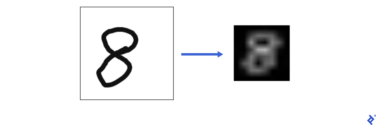
Now, it’s time to test our application. After starting the application, use the command below to send a request with this iStock image to the API:

1
2

export FLASK_APP=app
flask run

1

curl "http://localhost:5000/api/predict" -X "POST" -H "Content-Type: application/json" -d "{\"image\": \"data:image/png;base64,$(curl "https://media.istockphoto.com/vectors/number-eight-8-hand-drawn-with-dry-brush-vector-id484207302?k=6&m=484207302&s=170667a&w=0&h=s3YANDyuLS8u2so-uJbMA2uW6fYyyRkabc1a6OTq7iI=" | base64)\"}" -i

You should see the following output:

1
2
3
4
5
6
7
8
9

HTTP/1.1 100 Continue

HTTP/1.0 200 OK
Content-Type: text/html; charset=utf-8
Content-Length: 1
Server: Werkzeug/0.14.1 Python/3.6.3
Date: Tue, 27 Mar 2018 07:02:08 GMT

8

Our application successfully identified the digit ‘8’ from the sample image.

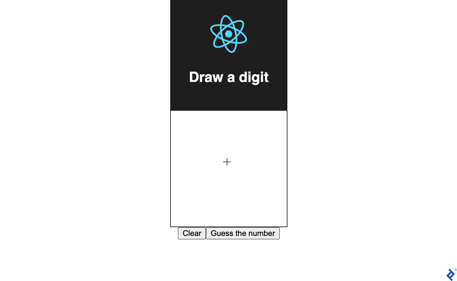
Building a Drawing Interface with React

To quickly set up the front-end, we’ll use CRA boilerplate:

1
2

create-react-app frontend
cd frontend

Next, we need a dependency for drawing digits. The react-sketch package perfectly suits our requirements:

1

npm i react-sketch

Our application comprises a single component with two main aspects: logic and view.

The view is responsible for rendering the drawing canvas, along with Submit and Reset buttons. It also displays predictions or errors. On the logic side, we handle image submission and sketch clearing.

Clicking Submit triggers the extraction of the drawn image, which is then sent to the API’s makePrediction function. Successful requests update the prediction state, while errors are reflected in the error state.

Clicking Reset clears the drawing canvas:

 1
 2
 3
 4
 5
 6
 7
 8
 9
10
11
12
13
14
15
16
17
18
19
20
21
22

import React, { useRef, useState } from "react";

import { makePrediction } from "./api";

const App = () => {
  const sketchRef = useRef(null);
  const [error, setError] = useState();
  const [prediction, setPrediction] = useState();

  const handleSubmit = () => {
    const image = sketchRef.current.toDataURL();

    setPrediction(undefined);
    setError(undefined);

    makePrediction(image).then(setPrediction).catch(setError);
  };

  const handleClear = (e) => sketchRef.current.clear();

  return null
}

With the logic in place, let’s add the visual elements:

 1
 2
 3
 4
 5
 6
 7
 8
 9
10
11
12
13
14
15
16
17
18
19
20
21
22
23
24
25
26
27
28
29
30
31
32
33
34
35
36
37
38
39
40
41
42
43
44
45
46
47
48
49
50
51
52
53
54
55
56
57
58
59
60
61
62
63
64
65
66
67
68
69
70

import React, { useRef, useState } from "react";
import { SketchField, Tools } from "react-sketch";

import { makePrediction } from "./api";

import logo from "./logo.svg";
import "./App.css";

const pixels = (count) => `${count}px`;
const percents = (count) => `${count}%`;

const MAIN_CONTAINER_WIDTH_PX = 200;
const MAIN_CONTAINER_HEIGHT = 100;
const MAIN_CONTAINER_STYLE = {
  width: pixels(MAIN_CONTAINER_WIDTH_PX),
  height: percents(MAIN_CONTAINER_HEIGHT),
  margin: "0 auto",
};

const SKETCH_CONTAINER_STYLE = {
  border: "1px solid black",
  width: pixels(MAIN_CONTAINER_WIDTH_PX - 2),
  height: pixels(MAIN_CONTAINER_WIDTH_PX - 2),
  backgroundColor: "white",
};

const App = () => {
  const sketchRef = useRef(null);
  const [error, setError] = useState();
  const [prediction, setPrediction] = useState();

  const handleSubmit = () => {
    const image = sketchRef.current.toDataURL();

    setPrediction(undefined);
    setError(undefined);

    makePrediction(image).then(setPrediction).catch(setError);
  };

  const handleClear = (e) => sketchRef.current.clear();

  return (
    <div className="App" style={MAIN_CONTAINER_STYLE}>
      <div>
        <header className="App-header">
          <img src={logo} className="App-logo" alt="logo" />
          <h1 className="App-title">Draw a digit</h1>
        </header>
        <div style={SKETCH_CONTAINER_STYLE}>
          <SketchField
            ref={sketchRef}
            width="100%"
            height="100%"
            tool={Tools.Pencil}
            imageFormat="jpg"
            lineColor="#111"
            lineWidth={10}
          />
        </div>
        {prediction && <h3>Predicted value is: {prediction}</h3>}
        <button onClick={handleClear}>Clear</button>
        <button onClick={handleSubmit}>Guess the number</button>
        {error && <p style={{ color: "red" }}>Something went wrong</p>}
      </div>
    </div>
  );
};

export default App;

Our component is now complete. To test it, execute the following command and navigate to localhost:3000 in your web browser:

1

npm run start

A live demo of the application is accessible here. You can also explore the source code on GitHub.

Conclusion

While the accuracy of our digit classifier might not be flawless, that was not our primary objective. The disparity between the training data and user-drawn input is significant. Nonetheless, we managed to build a functional application from scratch in under 30 minutes.

Through this process, we gained valuable experience in:

• Machine learning
• Back-end development
• Image processing
• Front-end development

Software capable of recognizing handwritten digits finds applications in diverse domains, from education and administration to postal and financial services.

Hopefully, this article inspires you to further explore machine learning, image processing, and front-end and back-end development, using these skills to craft innovative and impactful applications.

For those interested in deepening their understanding of machine learning and image processing, our Adversarial Machine Learning Tutorial is a valuable resource.