Computers and their processors excel at working with numbers, yet everyday language, like that found in emails and social media, lacks a structured format suitable for computation.

This is where natural language processing (NLP) bridges the gap. NLP, a field within computer science intersecting with linguistics, employs computational methods, particularly artificial intelligence, to decipher natural language and speech. Topic modeling, a key aspect of NLP, aims to determine the subjects covered within a given text. This capability empowers developers to create valuable features, including real-time detection of breaking news on social media platforms, personalized message recommendations, identification of fake user accounts, and analysis of information dissemination patterns.

How can developers enable computers, primarily designed for calculations, to grasp human communication at such advanced levels?

Representing Text Mathematically: The Bag of Words Model

To address this, we need a way to represent text mathematically. Our journey in this Python topic-modeling tutorial begins with the most straightforward approach: the bag of words model.

In this model, a text is represented simply as a collection of its words, disregarding grammar and even word order but keeping multiplicity. For instance, the sentence This is an example can be represented by the set of words it contains, along with their counts:

1

{"an": 1, "example": 1, "is": 1, "this": 1}

Notice that this method disregards word order. Consider the following:

• “I like Star Wars but I don’t like Harry Potter.”
• “I like Harry Potter but I don’t like Star Wars.”

Though these sentences express opposing sentiments, they share the same words. For the purpose of topic analysis, this difference is inconsequential as both sentences revolve around preferences for Harry Potter and Star Wars. Thus, word order is irrelevant in this context.

When dealing with multiple texts and aiming to understand their disparities, a mathematical representation of the entire corpus is required, treating each text individually. A matrix proves suitable, where each column corresponds to a unique word and each row represents a text. One possible corpus representation involves populating each cell with the frequency of a particular word (column) appearing in a specific text (row).

In our example, the corpus comprises two sentences, forming the rows of our matrix:

1
2

["I like Harry Potter",
"I like Star Wars"]

The words in our corpus are listed in the order of their appearance: I, like, Harry, Potter, Star, Wars. These words constitute the columns of our matrix.

The matrix values represent the count of each word within each phrase:

1
2

[[1,1,1,1,0,0],
[1,1,0,0,1,1]]

The matrix size is determined by the product of the number of texts and the number of distinct words present in at least one text. The latter often yields an unnecessarily large matrix, which can be optimized. For example, a matrix might have separate columns for “play” and “played” despite their semantic similarity.

Conversely, columns representing novel concepts might be absent. “Classical” and “music” each carry individual meanings, but their combination, “classical music,” introduces a new concept.

These limitations necessitate text preprocessing for optimal results.

Refining Analysis Through Preprocessing and Topic Clustering Models

Achieving optimal results often involves employing various preprocessing techniques. Let’s delve into some commonly used ones:

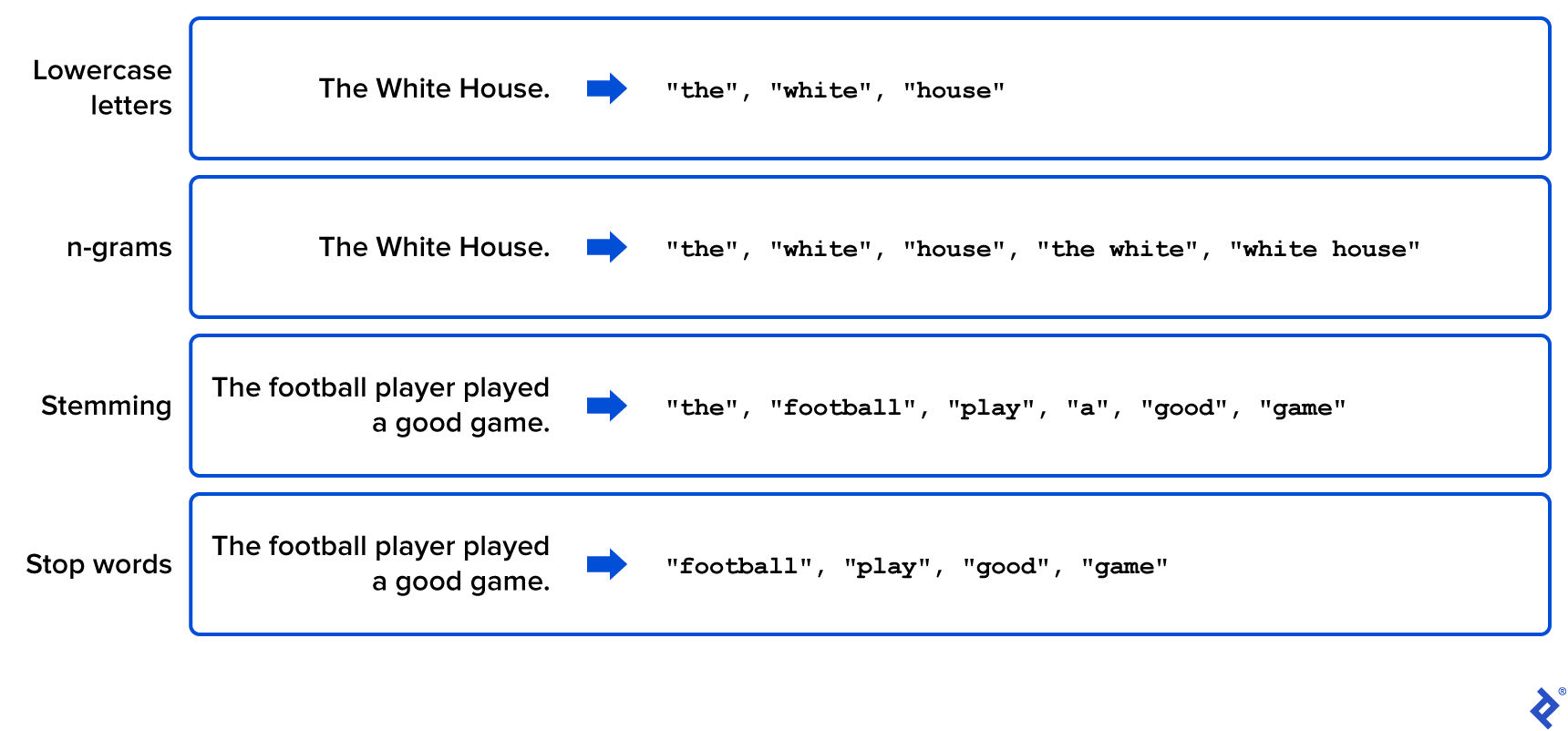
1. Lowercase Conversion: Standardize all words to lowercase. This eliminates variations stemming from capitalization, as the meaning remains consistent.

2. n-grams: Treat consecutive groups of n words as single terms, called n-grams. This captures phrases like “white house,” adding them to the vocabulary list.

3. Stemming: Isolate word roots by identifying and removing prefixes and suffixes. For instance, “play,” “played,” and “player” would all be represented by the stem “play.” While stemming can shrink the vocabulary size without significant information loss, it increases preprocessing time due to its application to each word.

4. Stop Word Removal: Eliminate words lacking substantial meaning or utility, such as articles, prepositions, and potentially other words irrelevant to the specific analysis, such as certain common verbs.

5. Term Frequency–Inverse Document Frequency (tf–idf): Instead of raw frequency counts, use the tf–idf coefficient, calculated by multiplying two values:

   • tf: The frequency of a term within a text.
   • idf: The logarithm of the total number of documents divided by the number of documents containing that term.

   tf–idf measures a word’s importance within a corpus. Distinguishing topics requires understanding not only word presence but also words frequent in one text but absent in others.

The following illustration provides simple examples of these preprocessing techniques, showcasing how the corpus’s original text is transformed to create a focused and manageable word list:

Let’s illustrate the application of some of these techniques using Python. With a mathematical representation of our corpus, we can then uncover discussed topics by applying unsupervised machine learning algorithms. “Unsupervised” signifies that the algorithm operates without predefined topic labels, such as “science fiction.”

Several algorithms can cluster our corpus, including non-negative matrix factorization (NMF), sparse principal components analysis (sparse PCA), and latent dirichlet allocation (LDA). We’ll concentrate on LDA due to its popularity in the scientific community, stemming from its effectiveness in areas like social media, medical science, political science, and software engineering.

LDA is an unsupervised topic decomposition model, grouping texts based on word content and the probability of a word belonging to a particular topic. The LDA algorithm generates the topic word distribution. This distribution allows us to define the main topics based on their most likely associated words. Once we identify the main topics and their related words, we can determine which topic(s) apply to each text.

Consider the following corpus comprising five short sentences (all extracted from New York Times headlines):

1
2
3
4
5

corpus = [ "Rafael Nadal Joins Roger Federer in Missing U.S. Open",
          "Rafael Nadal Is Out of the Australian Open",
          "Biden Announces Virus Measures",
          "Biden's Virus Plans Meet Reality",
          "Where Biden's Virus Plan Stands"]

The algorithm should readily identify one topic related to politics and coronavirus, and another related to Nadal and tennis.

Implementing the Strategy Using Python

To detect these topics, we need to import the necessary libraries. Python offers powerful libraries for NLP and machine learning, including NLTK and Scikit-learn (sklearn).

1
2
3
4

from sklearn.feature_extraction.text import CountVectorizer
from sklearn.feature_extraction.text import TfidfTransformer
from sklearn.decomposition import LatentDirichletAllocation as LDA
from nltk.corpus import stopwords

Utilizing CountVectorizer(), we construct the word frequency matrix for each text. Note that CountVectorizer() allows preprocessing through parameters like stop_words for including stop words, ngram_range for incorporating n-grams, and lowercase=True for converting all characters to lowercase.

1
2
3
4
5
6
7
8
9

count_vect = CountVectorizer(stop_words=stopwords.words('english'), lowercase=True)
x_counts = count_vect.fit_transform(corpus)
x_counts.todense()

matrix([[0, 0, 0, 1, 1, 0, 0, 1, 1, 1, 0, 0, 1, 0, 1, 0, 0],
        [0, 1, 0, 0, 0, 0, 0, 0, 1, 1, 0, 0, 1, 0, 0, 0, 0],
        [1, 0, 1, 0, 0, 1, 0, 0, 0, 0, 0, 0, 0, 0, 0, 0, 1],
        [0, 0, 1, 0, 0, 0, 1, 0, 0, 0, 0, 1, 0, 1, 0, 0, 1],
        [0, 0, 1, 0, 0, 0, 0, 0, 0, 0, 1, 0, 0, 0, 0, 1, 1]], dtype=int64)

To define our corpus vocabulary, we can simply use the .get_feature_names() attribute:

1
2
3

count_vect.get_feature_names()

['announces', 'australian', 'biden', 'federer', 'joins', 'measures', 'meet', 'missing', 'nadal', 'open',  'plan', 'plans', 'rafael', 'reality', 'roger', 'stands', 'virus']

Next, we perform tf–idf calculations using the sklearn function:

1
2

tfidf_transformer = TfidfTransformer()
x_tfidf = tfidf_transformer.fit_transform(x_counts)

Before executing LDA decomposition, we must specify the number of topics. In this straightforward scenario, we know there are two topics or “dimensions.” However, in more complex cases, this becomes a hyperparameter that needs some tuning, potentially using algorithms like random search or grid search:

 1
 2
 3
 4
 5
 6
 7
 8
 9
10

dimension = 2
lda = LDA(n_components = dimension)
lda_array = lda.fit_transform(x_tfidf)
lda_array

array([[0.8516198 , 0.1483802 ],
       [0.82359501, 0.17640499],
       [0.18072751, 0.81927249],
       [0.1695452 , 0.8304548 ],
       [0.18072805, 0.81927195]])

LDA is inherently probabilistic. The output shows the probability of each of the five headlines belonging to each of the two topics. As expected, the first two texts exhibit a higher probability of belonging to the first topic, while the remaining three lean towards the second topic.

Finally, to understand the content of these two topics, we can examine the most significant words within each:

1
2
3
4
5
6

components = [lda.components_[i] for i in range(len(lda.components_))]
features = count_vect.get_feature_names()
important_words = [sorted(features, key = lambda x: components[j][features.index(x)], reverse = True)[:3] for j in range(len(components))]
important_words
[['open', 'nadal', 'rafael'], 
['virus', 'biden', 'measures']]

As anticipated, LDA accurately assigned words related to tennis tournaments and Nadal to the first topic and words associated with Biden and the virus to the second.

Scaling Up: Large-scale Analyses and Real-world Applications

A compelling example of large-scale topic modeling analysis can be found in this paper. The study investigated major news topics during the 2016 US presidential election, observing topics covered by prominent media outlets like the New York Times and Fox News, including corruption and immigration. Furthermore, the paper examined correlations and causations between media content and election outcomes.

Topic modeling finds extensive application beyond academia, proving invaluable for uncovering hidden topical patterns within massive text collections. For example, it plays a crucial role in recommendation systems and helps determine customer/user sentiment and discussion points from surveys, feedback forms, and social media interactions.

The Toptal Engineering Blog expresses its gratitude to Juan Manuel Ortiz de Zarate for reviewing the code samples presented in this article.

Further Exploration: Recommended Reading on Topic Modeling

Improved Topic Modeling in Twitter Albanese, Federico and Esteban Feuerstein. “Improved Topic Modeling in Twitter Through Community Pooling.” (December 20, 2021): arXiv:2201.00690 [cs.IR] Analyzing Twitter for Public Health Paul, Michael and Mark Dredze. “You Are What You Tweet: Analyzing Twitter for Public Health.” August 3, 2021. Classifying Political Orientation on Twitter Cohen, Raviv and Derek Ruths. “Classifying Political Orientation on Twitter: It’s Not Easy!” August 3, 2021. Using Relational Topic Models to Capture Coupling Gethers, Malcolm and Denis Poshyvanyk. “Using Relational Topic Models to Capture Coupling Among Classes in Object-oriented Software Systems.” October 25, 2010.