Let’s explore reinforcement learning by tackling a practical problem using popular libraries such as TensorFlow, TensorBoard, Keras, and OpenAI Gym. We’ll implement deep $Q$-learning to understand its workings. The code will run on a standard PC, leveraging all CPU cores thanks to TensorFlow’s capabilities.

Our problem is the Mountain Car: Imagine a car on a one-dimensional track between two mountains. The goal is to drive up the right mountain (reaching a flag). However, the car’s engine is weak and cannot climb the mountain directly. Success requires building momentum by driving back and forth.

This problem is ideal for our purpose because it’s simple enough for reinforcement learning to solve quickly on a single CPU core yet complex enough to demonstrate the core concepts.

First, we’ll briefly overview reinforcement learning. We’ll then define basic terms and frame our problem using them. Next, we’ll delve into the deep $Q$-learning algorithm and implement it to solve the Mountain Car problem.

Fundamentals of Reinforcement Learning

Reinforcement learning, simply put, is learning through trial and error. The central entity is an “agent,” which is our car in this scenario. The agent interacts with an environment by taking actions. For each action, it receives feedback in the form of a new observation and a reward. Actions leading to higher rewards are encouraged, hence the term “reinforcement.” This concept draws inspiration from observing how living beings learn.

The agent’s interactions within the environment are depicted in the following diagram:

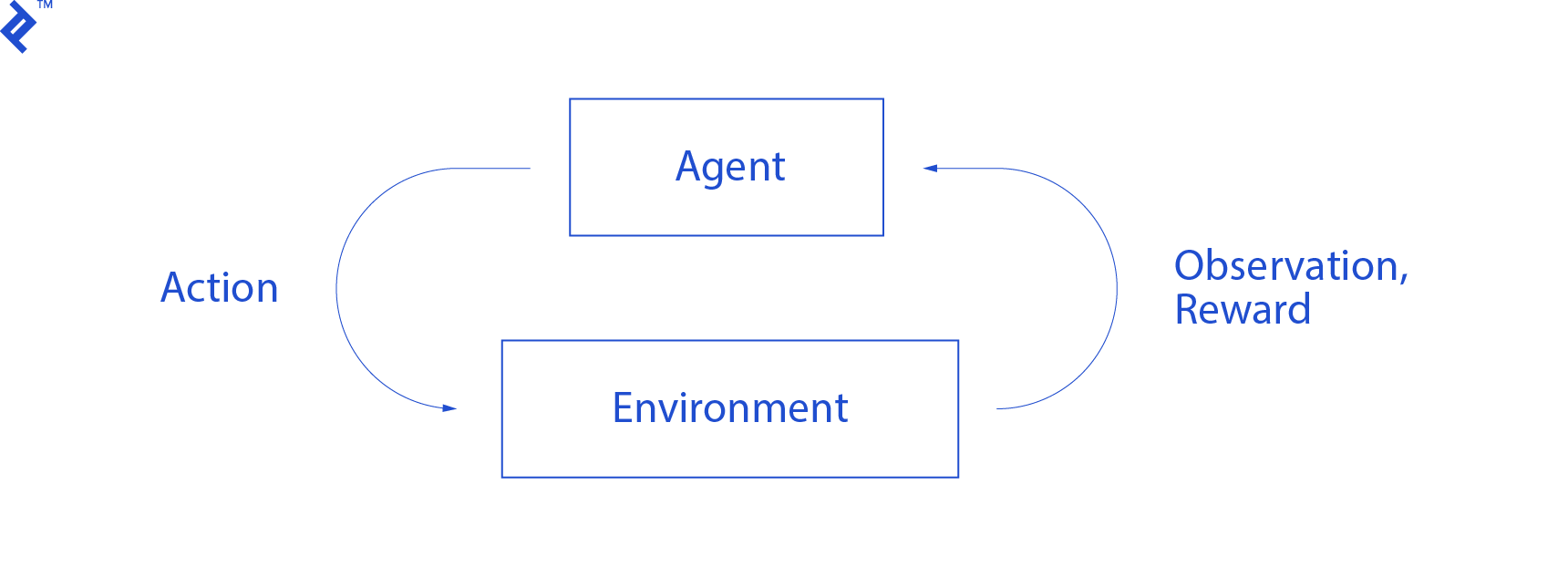
The agent perceives an observation and receives a reward based on its action. It then chooses another action, leading to step two. The environment responds with potentially altered observations and rewards. This cycle repeats until a terminal state is reached, signaled by a “done” notification sent to the agent. The complete sequence of observations > actions > next_observations > rewards is called an episode (or trajectory).

Returning to our Mountain Car: The car represents our agent, while the one-dimensional mountainous terrain acts as the environment. The car’s action is represented by a single number: a positive value signifies pushing the car right, and a negative value signifies pushing it left. The agent perceives its surroundings through observations: the car’s X position and velocity. To guide the car to the mountaintop, we define the reward accordingly: The agent receives a -1 reward for each step where it hasn’t reached the goal. Upon reaching the goal, the episode concludes. This setup effectively penalizes the agent for not being in the desired position, encouraging it to reach the goal as swiftly as possible. The agent aims to maximize its total reward, which is the sum of rewards earned within an episode. For instance, reaching the goal after 110 steps yields a total return of -110, considered a favorable outcome for the Mountain Car problem. Failure to reach the goal within 200 steps results in a -200 return.

With the problem formulated, we can employ algorithms capable of solving it efficiently (when properly configured). It’s crucial to note that we don’t explicitly instruct the agent on how to achieve the goal; we provide no hints or heuristics. The agent is left to discover its own winning strategy (policy).

Setting Up the Environment

Begin by downloading the entire tutorial code:

1
2

git clone https://github.com/AdamStelmaszczyk/rl-tutorial
cd rl-tutorial

Next, we’ll install the necessary Python packages. To prevent conflicts with existing installations, we’ll create a clean conda environment. If you haven’t installed conda, please refer to https://conda.io/docs/user-guide/install/index.html.

To create the conda environment:

1

conda create -n tutorial python=3.6.5 -y

Activate it using:

1

source activate tutorial

You should now see (tutorial) near your shell prompt, indicating the activation of the “tutorial” conda environment. Execute all subsequent commands within this environment.

Install the required dependencies within the conda environment:

1

pip install -r requirements.txt

With the installation complete, let’s execute some code. We don’t need to implement the Mountain Car environment from scratch, as the OpenAI Gym library provides a ready-made implementation. Let’s observe a random agent (an agent selecting random actions) in our environment:

 1
 2
 3
 4
 5
 6
 7
 8
 9
10
11
12
13
14
15
16
17
18
19
20
21

import gym

env = gym.make('MountainCar-v0')
done = True
episode = 0
episode_return = 0.0
for episode in range(5):
   for step in range(200):
       if done:
           if episode > 0:
               print("Episode return: ", episode_return)
           obs = env.reset()
           episode += 1
           episode_return = 0.0
           env.render()
       else:
           obs = next_obs
       action = env.action_space.sample()
       next_obs, reward, done, _ = env.step(action)
       episode_return += reward
       env.render()

This is the see.py file. Execute it using:

1

python see.py

You should see the car moving randomly back and forth. Each episode will last 200 steps, resulting in a total return of -200.

Now, we need to replace these random actions with a more effective strategy. Numerous algorithms can be employed; deep $Q$-learning is well-suited for this introductory tutorial. Understanding this method provides a strong foundation for exploring other approaches.

Deep $Q$-learning

We will be using the algorithm first presented in 2013 by Mnih et al. in Playing Atari with Deep Reinforcement Learning and refined two years later in Human-level control through deep reinforcement learning. These papers have spawned many advancements in the field, including the current state-of-the-art algorithm Rainbow (2017):

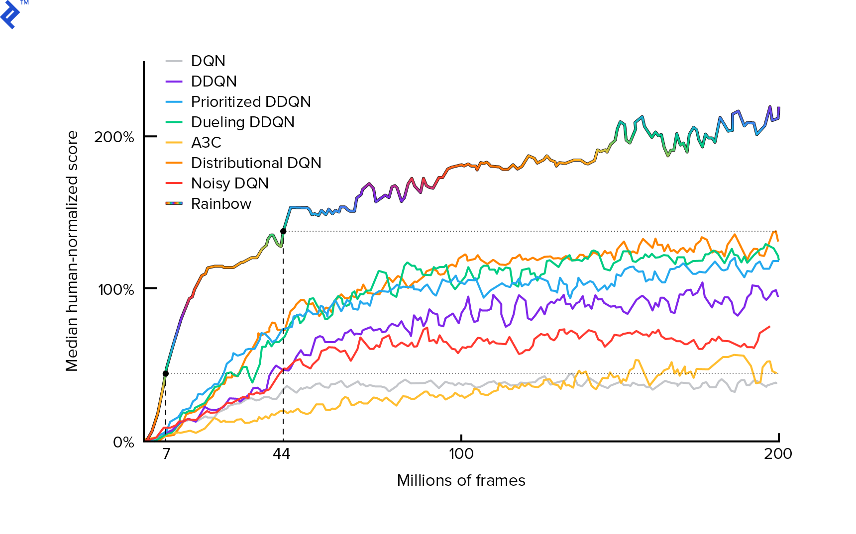
Rainbow achieves superhuman performance in many Atari 2600 games. We’ll concentrate on the fundamental DQN version with minimal enhancements to keep this tutorial concise.

A policy, often denoted as $π(s)$, is a function that outputs the probabilities of taking specific actions in a given state $s$. For instance, a random Mountain Car policy would always return a 50% chance for both left and right actions in any state. During gameplay, we sample from this policy (distribution) to determine the actual actions taken.

$Q$-learning (Q stands for Quality) refers to the action-value function, denoted as $Q_π(s, a)$. This function returns the expected total return when starting in state $s$, taking action $a$, and then following the policy $π$. The total return represents the sum of all rewards obtained during an episode.

Knowing the optimal $Q$-function, represented as $Q^*$, would make solving the game trivial. We would simply select actions associated with the highest $Q^*$ values, guaranteeing the highest possible return.

However, $Q^*$ is usually unknown. In such cases, we can approximate or “learn” it through interactions with the environment. This is the essence of “$Q$-learning.” The term “deep” comes from utilizing deep neural networks, versatile function approximators, to approximate this function. Deep neural networks used for this purpose are known as Deep Q-Networks (DQNs). In simpler environments (where the number of states is manageable), a table could be used instead of a neural network to represent the $Q$-function, leading to “tabular $Q$-learning.”

Our goal is to approximate the $Q^*$ function. The Bellman equation aids us in this endeavor:

[Q(s, a) = r + γ \space \textrm{max}_{a’} Q(s’, a’)]

$s’$ represents the state reached after taking action $a$ in state $s$. $γ$ (gamma), often set to 0.99, is a discount factor (a hyperparameter). It assigns less weight to future rewards, as they are less certain than immediate rewards given our imperfect $Q$. The Bellman equation is pivotal in deep $Q$-learning. It states that the $Q$-value for a specific state and action equals the immediate reward $r$ plus the discounted maximum $Q$-value achievable from the next state $s’$. We select the action $a’$ that leads to the highest total return from $s’$.

Leveraging the Bellman equation, we can employ supervised learning to approximate $Q^*$. The $Q$-function is represented (parametrized) by the neural network weights, denoted as $θ$ (theta). A naive implementation might take a state and an action as input and output the corresponding $Q$-value. However, this becomes inefficient when we need to know the $Q$-values for all actions in a given state, requiring as many calls to the $Q$ function as there are actions. A more efficient approach is to input only the state and obtain $Q$-values for all possible actions as output. This allows us to retrieve all $Q$-values in a single forward pass.

We begin by initializing the $Q$ network with random weights. As the agent interacts with the environment, we collect numerous transitions or “experiences.” These are tuples of (state, action, next state, reward), often abbreviated as ($s$, $a$, $s’$, $r$). We store thousands of these experiences in a ring buffer known as the “experience replay.” Experiences are then sampled from this buffer, aiming to fulfill the Bellman equation. Although we could process experiences one by one (online or on-policy learning), consecutive experiences tend to be highly correlated, hindering DQN training. The experience replay (offline or off-policy learning) mitigates this issue by disrupting data correlation. The replay_buffer.py file contains a straightforward ring buffer implementation that is worth examining.

Initially, with random neural network weights, the left-hand side of the Bellman equation will deviate significantly from the right-hand side. We use the squared difference as our loss function and minimize it by adjusting the neural network weights $θ$. The loss function can be expressed as:

[L(θ) = [Q(s, a) - r - γ \space \textrm{max}_{a’}Q(s’, a’)]^2]

This is simply a rearrangement of the Bellman equation. For example, suppose we sample the experience ($s$, left, $s’$, -1) from the Mountain Car experience replay. We pass state $s$ through our $Q$ network, and let’s say it outputs -120 for the left action, so $Q(s, \textrm{left}) = -120$. Next, we input $s’$ to the network, yielding -130 for left and -122 for right. Clearly, the better action for $s’$ is right, resulting in $\textrm{max}_{a’}Q(s’, a’) = -122$. We know $r$, the actual reward, which was -1. This means our $Q$-network’s prediction was slightly off, as $L(θ) = [-120 - 1 + 0.99 ⋅ 122]^2 = (-0.22^2) = 0.0484$. We then backpropagate the error to adjust the weights $θ$. If we recalculate the loss for the same experience, it would now be lower.

One crucial observation before diving into the code: Updating our DQN involves two forward passes through the same network, which can lead to unstable learning. To address this, we use a slightly older version of the network, referred to as target_model (as opposed to the main DQN, model), to predict the next state $Q$ values. This provides a stable target. We synchronize target_model with the weights of model every 1000 steps, while model is updated after each step.

Let’s examine the code responsible for creating the DQN model:

 1
 2
 3
 4
 5
 6
 7
 8
 9
10
11
12
13

def create_model(env):
   n_actions = env.action_space.n
   obs_shape = env.observation_space.shape
   observations_input = keras.layers.Input(obs_shape, name='observations_input')
   action_mask = keras.layers.Input((n_actions,), name='action_mask')
   hidden = keras.layers.Dense(32, activation='relu')(observations_input)
   hidden_2 = keras.layers.Dense(32, activation='relu')(hidden)
   output = keras.layers.Dense(n_actions)(hidden_2)
   filtered_output = keras.layers.multiply([output, action_mask])
   model = keras.models.Model([observations_input, action_mask], filtered_output)
   optimizer = keras.optimizers.Adam(lr=LEARNING_RATE, clipnorm=1.0)
   model.compile(optimizer, loss='mean_squared_error')
   return model

This function begins by retrieving the action and observation space dimensions from the OpenAI Gym environment. This information is crucial, determining factors such as the number of outputs for our network (equal to the number of actions). Actions are one-hot encoded:

1
2
3
4

def one_hot_encode(n, action):
   one_hot = np.zeros(n)
   one_hot[int(action)] = 1
   return one_hot

For example, left becomes [1, 0] and right becomes [0, 1].

Observe that we input the observations. We also provide action_mask as a second input. This is because, when calculating $Q(s,a)$, we are only interested in the $Q$-value for a single specific action, not all of them. action_mask contains a 1 for the action whose $Q$-value we want to retrieve from the DQN output. If action_mask has a 0 for a particular action, its corresponding $Q$-value is zeroed out at the output. The filtered_output layer handles this. When we need all $Q$-values (for the max calculation), we can simply pass a vector of ones.

The code utilizes keras.layers.Dense to define fully connected layers. Keras is a Python library that provides a higher-level abstraction over TensorFlow. Behind the scenes, Keras constructs a TensorFlow graph with biases, weight initialization, and other low-level details. While we could have used raw TensorFlow to define the graph, Keras simplifies this process significantly.

Observations are passed through the first hidden layer, which uses ReLU (rectified linear unit) activations. ReLU(x) is simply the $\textrm{max}(0, x)$ function. This layer is fully connected to a second identical layer, hidden_2. Finally, the output layer reduces the number of neurons to match the number of actions. The filtered_output layer then multiplies the output by action_mask.

To determine the optimal $θ$ weights, we employ the Adam optimizer with a mean squared error loss function.

With our model in place, we can predict $Q$ values for given state observations:

1
2
3

def predict(env, model, observations):
   action_mask = np.ones((len(observations), env.action_space.n))
   return model.predict(x=[observations, action_mask])

Here, we require $Q$-values for all actions, hence action_mask is a vector of ones.

The actual training is performed using the fit_batch() function:

 1
 2
 3
 4
 5
 6
 7
 8
 9
10
11
12
13
14
15
16

def fit_batch(env, model, target_model, batch):
   observations, actions, rewards, next_observations, dones = batch
   # Predict the Q values of the next states. Passing ones as the action mask.
   next_q_values = predict(env, target_model, next_observations)
   # The Q values of terminal states is 0 by definition.
   next_q_values[dones] = 0.0
   # The Q values of each start state is the reward + gamma * the max next state Q value
   q_values = rewards + DISCOUNT_FACTOR_GAMMA * np.max(next_q_values, axis=1)
   one_hot_actions = np.array([one_hot_encode(env.action_space.n, action) for action in actions])
   history = model.fit(
       x=[observations, one_hot_actions],
       y=one_hot_actions * q_values[:, None],
       batch_size=BATCH_SIZE,
       verbose=0,
   )
   return history.history['loss'][0]

Each batch contains BATCH_SIZE experiences. next_q_values represents $Q(s, a)$, while q_values represents $r + γ \space \textrm{max}_{a’}Q(s’, a’)$ from the Bellman equation. The actions taken are one-hot encoded and passed as action_mask during the model.fit() call. The variable $y$ typically represents the “target” in supervised learning, and we are setting it to q_values. The expression q_values[:. None] increases the array dimension to match the dimension of one_hot_actions. This is known as slice notation.

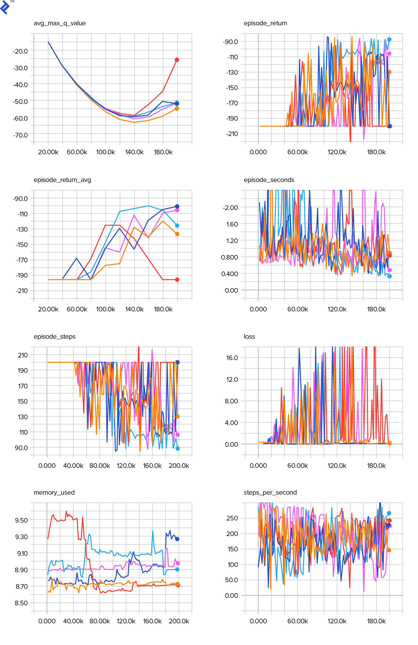
We return the loss value for logging in the TensorBoard log file, allowing us to visualize the training progress. Besides the loss, we also monitor other metrics such as steps per second, total RAM usage, and average episode return.

Running the Code

Before visualizing the TensorBoard log file, we need to generate it. Let’s begin training:

1

python run.py

This command first displays a summary of our model. It then creates a log directory named after the current date and initiates the training process. Every 2000 steps, a logline similar to this will be printed:

1

episode 10 steps 200/2001 loss 0.3346639 return -200.0 in 1.02s 195.7 steps/s 9.0/15.6 GB RAM

Every 20,000 steps, we evaluate the model’s performance over 10,000 steps:

1
2
3

Evaluation
100%|█████████████████████████████████████████████████████████████████████████████████| 10000/10000 [00:07<00:00, 1254.40it/s]
episode 677 step 120000 episode_return_avg -136.750 avg_max_q_value -56.004

After 677 episodes and 120,000 steps, the average episode return improved from -200 to -136.75, indicating that our agent is learning. Understanding the meaning of avg_max_q_value is left as a beneficial exercise. It’s a valuable statistic to observe during training.

The training concludes after 200,000 steps, taking approximately 20 minutes on a four-core CPU. Within the date-log directory (e.g., 06-07-18-39-log), you’ll find four model files with the .h5 extension. These files store snapshots of the TensorFlow graph weights, saved every 50,000 steps. They allow us to examine the learned policy later. To view it:

1

python run.py --model 06-08-18-42-log/06-08-18-42-200000.h5 --view

For additional options, use: python run.py --help.

Now, the car should navigate the track much more effectively, reaching the goal more consistently. Inside the date-log directory, there’s also an events.out.* file, where TensorBoard stores its data. We write to this file using the basic TensorBoardLogger defined in loggers.py. To visualize the events file, we need to launch a local TensorBoard server:

1

tensorboard --logdir=.

The --logdir flag points to the directory containing the date-log directories. In our case, it’s the current directory, so we use .. TensorBoard will print the URL it’s listening on. Open http://127.0.0.1:6006 in your web browser, and you should see eight plots resembling these:

Wrapping Up

The train() function handles the entire training process. First, it creates the model and initializes the replay buffer. Then, in a loop similar to the one in see.py, it interacts with the environment and stores experiences in the buffer. One key difference is that we follow an epsilon-greedy policy. While we could always select the best action according to the $Q$-function, this hinders exploration, which is crucial for overall performance. To enforce exploration, we choose random actions with epsilon probability:

 1
 2
 3
 4
 5
 6
 7
 8
 9
10
11

def greedy_action(env, model, observation):
   next_q_values = predict(env, model, observations=[observation])
   return np.argmax(next_q_values)


def epsilon_greedy_action(env, model, observation, epsilon):
   if random.random() < epsilon:
       action = env.action_space.sample()
   else:
       action = greedy_action(env, model, observation)
   return action

In this case, epsilon is set to 1%. Once 2000 experiences are collected, the replay buffer is sufficiently filled to commence training. We accomplish this by calling fit_batch() with a random batch of experiences sampled from the buffer:

1
2

batch = replay.sample(BATCH_SIZE)
loss = fit_batch(env, model, target_model, batch)

We evaluate the model’s performance and log the results every 20,000 steps (evaluation uses epsilon = 0, a purely greedy policy):

 1
 2
 3
 4
 5
 6
 7
 8
 9
10
11
12
13
14
15
16
17

if step >= TRAIN_START and step % EVAL_EVERY == 0:
   episode_return_avg = evaluate(env, model)
   q_values = predict(env, model, q_validation_observations)
   max_q_values = np.max(q_values, axis=1)
   avg_max_q_value = np.mean(max_q_values)
   print(
       "episode {} "
       "step {} "
       "episode_return_avg {:.3f} "
       "avg_max_q_value {:.3f}".format(
           episode,
           step,
           episode_return_avg,
           avg_max_q_value,
       ))
   logger.log_scalar('episode_return_avg', episode_return_avg, step)
   logger.log_scalar('avg_max_q_value', avg_max_q_value, step)

The entire codebase consists of approximately 300 lines, with run.py containing roughly 250 of the most important ones.

You might have noticed the numerous hyperparameters involved:

 1
 2
 3
 4
 5
 6
 7
 8
 9
10
11
12
13
14

DISCOUNT_FACTOR_GAMMA = 0.99
LEARNING_RATE = 0.001
BATCH_SIZE = 64
TARGET_UPDATE_EVERY = 1000
TRAIN_START = 2000
REPLAY_BUFFER_SIZE = 50000
MAX_STEPS = 200000
LOG_EVERY = 2000
SNAPSHOT_EVERY = 50000
EVAL_EVERY = 20000
EVAL_STEPS = 10000
EVAL_EPSILON = 0
TRAIN_EPSILON = 0.01
Q_VALIDATION_SIZE = 10000

This isn’t even an exhaustive list. Other factors, like network architecture, play a significant role as well. We used two hidden layers with 32 neurons, ReLU activations, and the Adam optimizer, but countless other configurations are possible. Even seemingly small adjustments can profoundly impact training. Fine-tuning hyperparameters often demands significant effort. In a recent OpenAI competition, the runner-up found out that it’s possible to almost double Rainbow’s score through meticulous hyperparameter optimization. However, it’s crucial to be mindful of overfitting. Currently, reinforcement learning algorithms struggle with generalizing knowledge to similar environments. Our Mountain Car agent, for instance, might not perform well on all types of mountains. You can experiment with modifying the OpenAI Gym environment to assess the agent’s generalization capabilities.

A worthwhile exercise is to try and discover a better set of hyperparameters than the ones used in this tutorial. However, judging the effectiveness of your changes based on a single training run is insufficient. Training runs often exhibit high variance, so multiple runs are necessary for meaningful comparisons. If you’re interested in learning more about the critical topic of reproducibility in machine learning, refer to Deep Reinforcement Learning that Matters. Instead of manual tuning, we can partially automate the hyperparameter optimization process, albeit at the cost of increased computational resources. A simple approach is to define a promising range for each hyperparameter and then perform a grid search (testing various combinations) with parallel training runs. Parallelization itself is a vast topic crucial for achieving high performance.

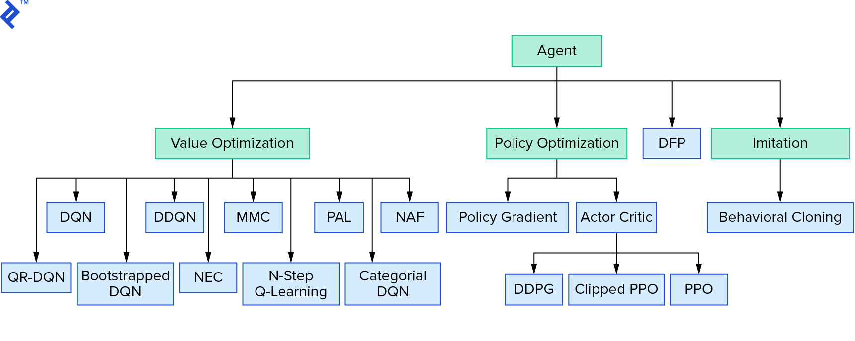
Deep $Q$-learning belongs to a broader family of reinforcement learning algorithms that rely on value iteration. We focused on approximating the $Q$-function and primarily used it greedily. Another family of algorithms utilizes policy iteration, aiming to directly find the optimal policy $π^*$ without explicitly approximating the $Q$-function. To see where value iteration fits within the broader landscape of reinforcement learning algorithms, refer to:

You might be thinking that deep reinforcement learning appears brittle, and you wouldn’t be wrong; it faces numerous challenges. For further reading on these challenges, see Deep Reinforcement Learning Doesn’t Work Yet and “Reinforcement Learning never worked, and ‘deep’ only helped a bit.”

This concludes our tutorial. We implemented a basic DQN for educational purposes. Very similar code can be used to achieve good performance in some Atari games. In practical applications, it’s common to leverage well-tested, high-performance implementations, such as those found in OpenAI baselines. If you’re interested in the hurdles of applying deep reinforcement learning to more complex environments, read Our NIPS 2017: Learning to Run approach. For a fun and competitive learning environment, explore platforms like NIPS 2018 Competitions or crowdai.org.

If your journey involves becoming a machine learning expert and you wish to expand your supervised learning expertise, consider exploring “Machine Learning Video Analysis: Identifying Fish” for an engaging fish identification experiment.