In our initial exploration of SQL indexes, we saw how sorting data could accelerate retrieval. However, sorting necessitates examining and rearranging each row, a process slower than a simple sequential table read.

This realization led us to the concept of maintaining sorted table duplicates, termed SQL indexes and prefixed with IX_. These indexes would facilitate the use of efficient retrieval algorithms without the need for pre-sorting.

The Index as a Sorted Table Replica

Let’s visualize this concept using Google Sheets, with our Reservation spreadsheet transformed into a collection of five sheets containing identical data. Each sheet within this setup is sorted based on different column combinations.

The following exercises, designed to be more intuitive than the previous SQL index tutorial, aim to illustrate:

1. Enhanced data retrieval efficiency using separate indexes over sorted primary tables
2. Order maintenance within indexes and tables during data modification

While our previous tutorial emphasized reads, real-world scenarios like hotel reservations necessitate considering indexing’s impact on write performance, encompassing both data insertion and updates.

Initial Exercise: Reservation Cancellation

To grasp SQL index performance with sorted tables, try deleting Client 12’s reservation for August 22nd, 2020, from Hotel 4. Remember to remove the row from all table copies while preserving correct sorting.

As you’ve likely observed, maintaining multiple sorted table copies is less than ideal. Inserting a new reservation or modifying an existing one further highlights this challenge.

Sorted copies, while aiding retrieval, complicate data modification. Adding, deleting, or updating necessitates retrieving all table copies, locating the relevant row and/or insertion point, and finally shifting data blocks.

SQL Indexes Employing Row Addresses

This spreadsheet showcases indexes utilizing a different approach. While maintaining sorted index rows based on specific criteria, these indexes only store the “row address,” indicating the row’s location within the Reservations sheet representing the main table, in column H.

Modern RDBMS implementations leverage operating system capabilities to swiftly locate disk blocks using physical addresses. Row addresses usually combine a block address with the row’s position within that block.

Let’s delve into some exercises to understand this index design.

Exercise 1: Retrieving All Reservations for a Client

Mirroring the first article, we’ll simulate the execution of this SQL query:

1
2
3

SELECT *
FROM Reservations
WHERE ClientID = 12;

Two approaches present themselves. The first involves reading all rows from the Reservations table and filtering for matches:

1
2

For each row from Reservations
  If Reservations.ClientID = 12 then write down Reservations.*

Alternatively, we can read data from the IX_ClientID sheet and, for each matching entry, locate the corresponding row in the Reservation table using the rowAddress value:

1
2
3
4
5
6

Get first row from IX_ClientID where ClientID = 12

While IX_ClientID.ClientID = 12
  Fetch Reservations.* where rowAddress = IX_ClientID.rowAddress
  Write down Reservations.*
  Get next row from IX_ClientID

Here, Get first row from is implemented via a loop similar to those previously encountered:

1
2
3

Repeat
  Fetch next row from IX_ClientID
Until ClientID >= 12

Locating a row using its rowAddress can be achieved by scrolling or filtering the rowAddress column.

For a small number of reservations, the index-based approach excels. However, with larger result sets (even tens of rows), directly querying the Reservations table might prove faster.

Read volume depends on the ClientID value. The largest value necessitates reading the entire index, while the smallest value resides at the beginning. The average case involves reading half the rows.

We’ll revisit this aspect later with a more efficient solution. For now, let’s focus on the steps after finding the first matching row.

Exercise 2: Counting Reservations Starting on a Specific Date

Our task is to count check-ins on August 16th, 2020, using the new index design.

1
2
3

SELECT COUNT (*)
FROM Reservations
WHERE DateFrom = TO_DATE('2020-08-16','YYYY-MM-DD');

When counting, the index-based approach surpasses a full table scan regardless of row count. This is because the index itself provides all necessary information:

1
2
3
4
5
6
7
8

Count := 0
Get first row from IX_DateFrom where DateFrom >= '2020-08-16'

While found and DateFrom < '2020-08-17'
  Count := Count + 1
  Get next row from IX_DateFrom

Write down Count

The algorithm resembles that for sorted tables. However, shorter index rows compared to table rows translate to fewer data blocks read from disk by the RDBMS.

Exercise 3: Guest List Retrieval Given Hotel and Date Range

Let’s generate a list of guests who arrived at Hotel 3 on August 13th and 14th, 2020.

1
2
3
4
5
6
7

SELECT ClientID
FROM Reservations
WHERE DateFrom BETWEEN (
    TO_DATE('2020-08-13','YYYY-MM-DD') AND
    TO_DATE('2020-08-14','YYYY-MM-DD')
  ) AND
  HotelID = 3;

We can either read all rows from the Reservations table or leverage an index. Our prior exercise with sorted tables revealed IX_HotelID_DateFrom as the most efficient index.

1
2
3
4
5
6
7
8

Get first row from IX_HotelID_DateFrom where
  HotelID = 3 and
  DateFrom between '2020-08-13' and '2020-08-14'

While found and DateFrom < '2020-08-15' and IX_HotelID_DateFrom.HotelID = 3
  Fetch Reservations.* where rowAddress = IX_HotelID_DateFrom.rowAddress
  Write down Reservations.ClientID
  Get next row from IX_HotelID_DateFrom

Designing a More Efficient Index

We access the table solely for the ClientID, the only information needed for our guest list. Including this value in the SQL index would eliminate table accesses altogether. Try generating the list solely from the IX_HotelID_DateFrom_ClientID index:

1
2
3
4
5
6
7

Get first row from IX_HotelID_DateFrom_ClientID where 
  HotelID = 3 and 
  DateFrom between '2020-08-13' and '2020-08-14'

While found and HotelID = 3 and DateFrom < '2020-08-15'
  Write down ClientID
  Get next row from IX_HotelID_DateFrom_ClientID

When an index contains all data required for query execution, it is said to cover the query.

Exercise 4: Retrieving Guest Names Instead of IDs

A list of guest IDs holds little value for criminal investigations. We need names:

1
2
3
4
5
6
7
8

SELECT c.ClientName
FROM Reservations r
JOIN Clients c ON r.ClientID = c.ClientID
WHERE r.DateFrom BETWEEN (
    TO_DATE('2020-08-13', 'YYYY-MM-DD') AND
    TO_DATE('2020-08-14', 'YYYY-MM-DD')
  ) AND
  r.HotelID = 3;

Besides the Reservations table, this necessitates accessing a Clients table containing guest information, found in this Google sheet.

This exercise mirrors the previous one, as does the approach.

1
2
3
4
5
6
7
8

Get first row from IX_HotelID_DateFrom_ClientID where 
  HotelID = 3 and 
  DateFrom between '2020-08-13' and '2020-08-14'

While found and HotelID = 3 and DateFrom < '2020-08-15' 
  Fetch Clients.* where ClientID = IX_HotelID_DateFrom_ClientID.ClientID
  Write down Clients.ClientName
  Get next row from IX_HotelID_DateFrom_ClientID

Implementing Fetch Clients.* where ClientID = IX_HotelID_DateFrom_ClientID.ClientID via table scan would require reading, on average, half the Clients table for each ClientID encountered in the While loop:

1
2
3
4
5
6

-- Get row from Clients using table scan
Repeat
  Fetch next row from Clients
Until ClientID = IX_HotelID_DateFrom_ClientID.ClientID or not found
If found
  Write down ClientName

Our current “flat” index implementation offers minimal benefit, requiring a similar number of reads (albeit from smaller rows) from the index, followed by jumps to Clients rows using RowAddress:

1
2
3
4
5
6
7

-- Get row from Clients using flat index
Repeat
  Fetch next row from Clients_PK_Flat
Until ClientID >= IX_HotelID_DateFrom_ClientID.ClientID
If found
  Fetch Clients.* where rowAddress = Clients_PK_Flat.rowAddress
  Write down ClientName

Note: PK denotes “primary key,” a concept we’ll explore further later in the series.

This begs the question: can we achieve this with fewer reads? The answer lies in B-tree indexes.

Balanced Tree (B-tree) Indexes

Let’s group rows from Clients_PK_Flat into four-row blocks, creating a list containing the last ClientID from each block and the block’s starting address (column IndexRowAddress). This new index structure, showcased in the Clients_PK_2Levels sheet, illustrates how to find a client with ClientID 28. The algorithm is as follows:

 1
 2
 3
 4
 5
 6
 7
 8
 9
10
11
12
13
14

Fetch Level2.*
Loop
  Leaf_address := Level3Address
  Exit when ClientID >= 28
  Fetch next row from Level2

Fetch Level3.* where Level3Address = Leaf_address -- 3-21
Loop
 Client_address := RowAddress
 Exit when ClientID >= 28
 Fetch next row from Level 3

Fetch Clients.* where rowAddress = Client_address -- 42
Write down Clients.*

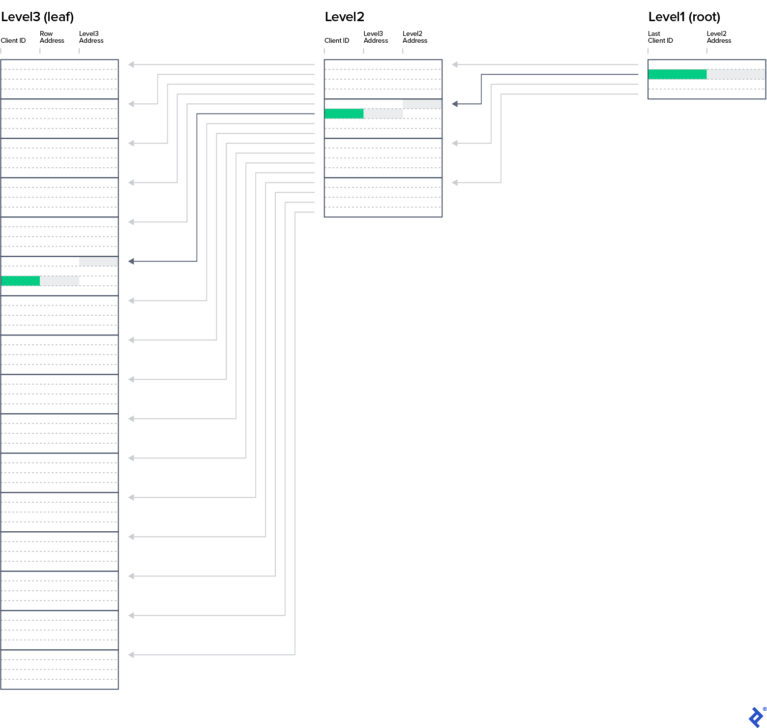
As you might have guessed, we can introduce another level. Level 1, comprising four rows, is visible in the IX_Clients_PK tab. Locating the name for ClientID 28 now requires reading three data blocks (nodes) – one per level – from the primary key structure, followed by a jump to the Clients row at address 42.

This SQL index structure is called a balanced tree. Balance is achieved when the path from the root node to each leaf-level node has the same length, known as the B-tree depth. Our example has a depth of three.

Henceforth, we’ll consider all indexes to have a B-tree structure, even though our spreadsheets only depict leaf-level entries. Key B-tree takeaways include:

• B-tree indexes are the most commonly used index by all major RDBMSs.
• All balanced tree levels are ordered by key column values.
• Data is read from disk in blocks.
• A single B-tree node can hold multiple blocks.
• Query performance heavily relies on the number of disk blocks read.
• The item count in each B-tree level, from root to leaf, increases exponentially.

Exercise 5: Enhanced Criminal Investigation

Our police inspector now seeks a list of guest names, arrival dates, and hotel names for all hotels in city A.

 1
 2
 3
 4
 5
 6
 7
 8
 9
10
11
12

SELECT
  h.HotelName,
  r.DateFrom as CheckInDate,
  c.ClientName
FROM Reservations r
JOIN Clients c ON r.ClientID = c.ClientID
JOIN Hotels h ON r.HotelID = h.HotelID
WHERE r.DateFrom BETWEEN (
    TO_DATE('2020-08-13', 'YYYY-MM-DD') AND
    TO_DATE('2020-08-14', 'YYYY-MM-DD')
  ) AND
  h.City = 'A';

Approach 1

Using the IX_DateFrom_HotelID_ClientID index would necessitate accessing the Hotels table for each date range row to check the hotel’s city. If it’s city A, we’d need to access the Clients table for the guest’s name.

 1
 2
 3
 4
 5
 6
 7
 8
 9
10

For each row from IX_DateFrom_HotelID_ClientID where
    DateFrom between '2020-08-13' and '2020-08-14'
  For each row from Hotels where
      HotelID = IX_DateFrom_HotelID_ClientID.HotelID
    If Hotels.City = 'A' then
      Fetch Clients.* where ClientID = IX_HotelID_DateFrom_ClientID.ClientID
      Write down
        Hotels.HotelName,
        IX_HotelID_DateFrom_ClientID.DateFrom,
        Clients.ClientName

Approach 2

IX_HotelID_DateFrom_ClientID offers a more efficient execution plan.

1
2
3
4
5
6
7
8
9

For each row from Hotels where City = 'A'
  For each row from IX_HotelID_DateFrom_ClientID where
      HotelID = Hotels.HotelID and
      DateFrom between '2020-08-13' and '2020-08-14'
    Fetch Clients.* where ClientID = IX_HotelID_DateFrom_ClientID.ClientID
    Write down
      Hotels.HotelName,
      IX_HotelID_DateFrom_ClientID.DateFrom,
      Clients.ClientName

We first retrieve all hotels in city A from the Hotels table. Using these hotel IDs, we then read subsequent entries from the IX_HotelID_DateFrom_ClientID index. This way, after locating the first B-tree leaf-level row for each hotel and date, we avoid reading reservations from hotels outside city A.

This highlights how a suitable database index can actually improve query speed despite an additional join.

The B-tree structure and its update mechanism upon row insertion, update, or deletion will be covered in greater detail when discussing partitioning’s rationale and impact. For now, consider this operation efficient when an index is employed.

SQL Index Queries: The Importance of Details

Working at the SQL level somewhat obscures underlying implementation details regarding indexes and databases. These exercises aimed to provide an intuitive understanding of execution plan behavior with different SQL indexes. Hopefully, you can now anticipate the optimal execution plan given available indexes and design indexes for maximum query efficiency.

The next installment in this series will build upon this newfound knowledge to explore common best practices and anti-patterns in SQL index usage. While I have a prepared list of topics, feel free to share your own questions to make the next article more relevant to your needs and experience.

The final part of SQL Indexes Explained will delve into table and index partitioning, examining the appropriate and inappropriate motivations for its use and its impact on query performance and database maintenance.