Enhance Your Data Cleaning Skills Using R

R is commonly known as a programming language used by statisticians and data scientists. While this was largely accurate in the past, the adaptability offered by R’s packages has transformed it into a more versatile language. Open sourced in 1995, R has experienced repositories of R packages are constantly growing since then. Nevertheless, R remains heavily data-centric compared to languages such as Python.

Among data types, tabular data stands out due to its widespread use. This format, resembling database tables, allows each column to hold a different data type. The efficiency of processing this data type is critical for many applications.

R can be used for very efficient data munging of tabular data

This article aims to demonstrate how to efficiently transform tabular data in R. Many R users, even those familiar with machine learning, are unaware that data munging can be achieved faster in R without relying on external tools.

High-Performance Tabular Data Transformation with R

Introduced in 1997, the data.frame class in base R, inherited from S-PLUS, stores data in memory in a column-oriented structure, unlike many databases that utilize row-by-row storage. This approach optimizes cache efficiency for column-based operations common in analytics. Additionally, R, despite being a functional programming language, doesn’t enforce this paradigm on developers. These advantages are effectively leveraged by the data.table R package, available in the CRAN repository. This package excels in grouping operations and memory efficiency by carefully materializing intermediate data subsets, generating only the columns required for a specific task. It also eliminates redundant copies through its reference semantics when adding or updating columns. First released in April 2006, the package significantly enhanced data.frame performance. The initial package description stated:

This package is intentionally minimal. Its sole purpose is to address the “white book” specification that data.frame must have row names. It introduces the data.table class, functionally similar to data.frame but with significantly reduced memory usage (up to 10 times less) and faster creation and copying (up to 10 times faster). Additionally, it enables subset() and with()-like expressions within []. Most of the code is adapted from base functions, removing row name manipulation.

Both data.frame and data.table have undergone improvements since then, but data.table continues to outperform base R significantly. In fact, it’s considered one of the fastest open-source data manipulation tools available, rivaling tools like Python Pandas and columnar databases or big data applications like Spark. Although benchmarks for its performance in distributed shared infrastructure are pending, its capacity to handle up to two billion rows on a single instance is promising. Its exceptional performance is attributed to its functionalities. Furthermore, ongoing efforts to parallelize time-consuming operations for incremental performance gains suggest a clear path for future optimization.

Illustrative Examples of Data Transformation

The interactive nature of R simplifies learning by allowing us to examine results at each step. Before proceeding, let’s install the data.table package from CRAN:

1
install.packages("data.table")

Helpful Tip: Access the manual for any function by prefixing its name with a question mark, for instance, ?install.packages.

Importing Data into R

R offers numerous packages for extracting data from various formats and databases, often including native drivers. In this example, we’ll load data from a CSV file, a prevalent format for raw tabular data. The file used in these examples is available here. We can rely on the highly optimized fread function for efficient CSV reading.

To utilize any function from a package, we need to load it using the library call:

1
2
3
library(data.table)
DT <- fread("flights14.csv")
print(DT)
 1
 2
 3
 4
 5
 6
 7
 8
 9
10
11
12
13
14
15
16
17
18
19
20
21
22
23
24
##         year month day dep_delay arr_delay carrier origin dest air_time
##      1: 2014     1   1        14        13      AA    JFK  LAX      359
##      2: 2014     1   1        -3        13      AA    JFK  LAX      363
##      3: 2014     1   1         2         9      AA    JFK  LAX      351
##      4: 2014     1   1        -8       -26      AA    LGA  PBI      157
##      5: 2014     1   1         2         1      AA    JFK  LAX      350
##     ---                                                                
## 253312: 2014    10  31         1       -30      UA    LGA  IAH      201
## 253313: 2014    10  31        -5       -14      UA    EWR  IAH      189
## 253314: 2014    10  31        -8        16      MQ    LGA  RDU       83
## 253315: 2014    10  31        -4        15      MQ    LGA  DTW       75
## 253316: 2014    10  31        -5         1      MQ    LGA  SDF      110
##         distance hour
##      1:     2475    9
##      2:     2475   11
##      3:     2475   19
##      4:     1035    7
##      5:     2475   13
##     ---              
## 253312:     1416   14
## 253313:     1400    8
## 253314:      431   11
## 253315:      502   11
## 253316:      659    8

If our data requires reshaping from long-to-wide or wide-to-long formats (also known as pivot and unpivot) for further processing, we can refer to the ?dcast and ?melt functions from the reshape2 package. However, data.table provides faster and more memory-efficient alternatives for data.table/data.frame objects.

Querying Data Using the data.table Syntax

If You Are Accustomed to data.frame

Querying data.table closely resembles querying data.frame. When filtering in the i argument, we can directly use column names without the need for the $ sign, as in df[df$col > 1, ]. The j argument accepts an expression to be evaluated within the scope of our data.table. To pass a non-expression j argument, use with=FALSE. The third argument, absent in the data.frame method, defines the groups, causing the expression in j to be evaluated by groups.

1
2
3
4
# data.frame
DF[DF$col1 > 1L, c("col2", "col3")]
# data.table
DT[col1 > 1L, .(col2, col3), ...] # by group using: `by = col4`

If You Are Familiar with Databases

Querying data.table shares similarities with SQL queries. DT in the example below symbolizes a data.table object and corresponds to SQL’s FROM clause.

1
2
3
4
5
6
DT[ i = where,
    j = select | update,
    by = group by]
  [ having, ... ]
  [ order by, ... ]
  [ ... ] ... [ ... ]
Untangling Tabluar Data

Sorting Rows and Reordering Columns

Sorting data is essential for time series analysis and crucial for data extraction and presentation. Sorting can be achieved by providing the integer vector of row order to the i argument, similar to data.frame. The first argument in the query order(carrier, -dep_delay) sorts data in ascending order based on the carrier field and descending order based on the dep_delay measure. The second argument j, as explained earlier, specifies the columns (or expressions) to be returned and their order.

1
2
3
ans <- DT[order(carrier, -dep_delay),
          .(carrier, origin, dest, dep_delay)]
head(ans)
1
2
3
4
5
6
7
##    carrier origin dest dep_delay
## 1:      AA    EWR  DFW      1498
## 2:      AA    JFK  BOS      1241
## 3:      AA    EWR  DFW      1071
## 4:      AA    EWR  DFW      1056
## 5:      AA    EWR  DFW      1022
## 6:      AA    EWR  DFW       989

To reorder data by reference instead of querying data in a specific order, we use the set* functions.

1
2
3
4
setorder(DT, carrier, -dep_delay)
leading.cols <- c("carrier","dep_delay")
setcolorder(DT, c(leading.cols, setdiff(names(DT), leading.cols)))
print(DT)
 1
 2
 3
 4
 5
 6
 7
 8
 9
10
11
12
13
14
15
16
17
18
19
20
21
22
23
24
##         carrier dep_delay year month day arr_delay origin dest air_time
##      1:      AA      1498 2014    10   4      1494    EWR  DFW      200
##      2:      AA      1241 2014     4  15      1223    JFK  BOS       39
##      3:      AA      1071 2014     6  13      1064    EWR  DFW      175
##      4:      AA      1056 2014     9  12      1115    EWR  DFW      198
##      5:      AA      1022 2014     6  16      1073    EWR  DFW      178
##     ---                                                                
## 253312:      WN       -12 2014     3   9       -21    LGA  BNA      115
## 253313:      WN       -13 2014     3  10       -18    EWR  MDW      112
## 253314:      WN       -13 2014     5  17       -30    LGA  HOU      202
## 253315:      WN       -13 2014     6  15        10    LGA  MKE      101
## 253316:      WN       -13 2014     8  19       -30    LGA  CAK       63
##         distance hour
##      1:     1372    7
##      2:      187   13
##      3:     1372   10
##      4:     1372    6
##      5:     1372    7
##     ---              
## 253312:      764   16
## 253313:      711   20
## 253314:     1428   17
## 253315:      738   20
## 253316:      397   16

In most cases, we only need either the original dataset or the ordered/sorted dataset. R, like other functional programming languages, by default returns sorted data as a new object, potentially doubling memory usage compared to sorting by reference.

Subset Queries

Let’s create a subset dataset for flights originating from “JFK” and departing between June and September. In the second argument, we limit the results to the listed columns, including a calculated variable sum_delay.

1
2
3
ans <- DT[origin == "JFK" & month %in% 6:9,
          .(origin, month, arr_delay, dep_delay, sum_delay = arr_delay + dep_delay)]
head(ans)
1
2
3
4
5
6
7
##    origin month arr_delay dep_delay sum_delay
## 1:    JFK     7       925       926      1851
## 2:    JFK     8       727       772      1499
## 3:    JFK     6       466       451       917
## 4:    JFK     7       414       450       864
## 5:    JFK     6       411       442       853
## 6:    JFK     6       333       343       676

When subsetting a dataset based on a single column, data.table automatically creates an index for that column. This results in real-time responses for subsequent filtering operations on that column.

Updating Datasets

Adding a new column by reference is performed using the := operator, which assigns a variable to the dataset in place. This avoids copying the dataset in memory, eliminating the need to assign results to a new variable.

1
2
DT[, sum_delay := arr_delay + dep_delay]
head(DT)
 1
 2
 3
 4
 5
 6
 7
 8
 9
10
11
12
13
14
##    carrier dep_delay year month day arr_delay origin dest air_time
## 1:      AA      1498 2014    10   4      1494    EWR  DFW      200
## 2:      AA      1241 2014     4  15      1223    JFK  BOS       39
## 3:      AA      1071 2014     6  13      1064    EWR  DFW      175
## 4:      AA      1056 2014     9  12      1115    EWR  DFW      198
## 5:      AA      1022 2014     6  16      1073    EWR  DFW      178
## 6:      AA       989 2014     6  11       991    EWR  DFW      194
##    distance hour sum_delay
## 1:     1372    7      2992
## 2:      187   13      2464
## 3:     1372   10      2135
## 4:     1372    6      2171
## 5:     1372    7      2095
## 6:     1372   11      1980

To add multiple variables simultaneously, use the syntax DT[, := (sum_delay = arr_delay + dep_delay)], similar to .(sum_delay = arr_delay + dep_delay) when querying the dataset.

Sub-assignment by reference, updating specific rows in place, is achieved by combining the i argument with the assignment operator.

1
2
3
DT[origin=="JFK",
   distance := NA]
head(DT)
 1
 2
 3
 4
 5
 6
 7
 8
 9
10
11
12
13
14
##    carrier dep_delay year month day arr_delay origin dest air_time
## 1:      AA      1498 2014    10   4      1494    EWR  DFW      200
## 2:      AA      1241 2014     4  15      1223    JFK  BOS       39
## 3:      AA      1071 2014     6  13      1064    EWR  DFW      175
## 4:      AA      1056 2014     9  12      1115    EWR  DFW      198
## 5:      AA      1022 2014     6  16      1073    EWR  DFW      178
## 6:      AA       989 2014     6  11       991    EWR  DFW      194
##    distance hour sum_delay
## 1:     1372    7      2992
## 2:       NA   13      2464
## 3:     1372   10      2135
## 4:     1372    6      2171
## 5:     1372    7      2095
## 6:     1372   11      1980

Aggregating Data

Data aggregation is performed by providing the third argument by to the square brackets. The j argument should contain aggregate function calls to perform the aggregation. The .N symbol used in the j argument represents the total number of observations within each group. As previously mentioned, aggregates can be combined with row subsets and column selections.

1
2
3
4
5
6
ans <- DT[,
          .(m_arr_delay = mean(arr_delay),
            m_dep_delay = mean(dep_delay),
            count = .N),
          .(carrier, month)]
head(ans)
1
2
3
4
5
6
7
##    carrier month m_arr_delay m_dep_delay count
## 1:      AA    10    5.541959    7.591497  2705
## 2:      AA     4    1.903324    3.987008  2617
## 3:      AA     6    8.690067   11.476475  2678
## 4:      AA     9   -1.235160    3.307078  2628
## 5:      AA     8    4.027474    8.914054  2839
## 6:      AA     7    9.159886   11.665953  2802

Comparing a row’s value to its group aggregate is a common requirement. In SQL, we use aggregates over partition by: AVG(arr_delay) OVER (PARTITION BY carrier, month).

1
2
3
4
5
ans <- DT[,
          .(arr_delay, carrierm_mean_arr = mean(arr_delay),
            dep_delay, carrierm_mean_dep = mean(dep_delay)),
          .(carrier, month)]
head(ans)
1
2
3
4
5
6
7
##    carrier month arr_delay carrierm_mean_arr dep_delay carrierm_mean_dep
## 1:      AA    10      1494          5.541959      1498          7.591497
## 2:      AA    10       840          5.541959       848          7.591497
## 3:      AA    10       317          5.541959       338          7.591497
## 4:      AA    10       292          5.541959       331          7.591497
## 5:      AA    10       322          5.541959       304          7.591497
## 6:      AA    10       306          5.541959       299          7.591497

To update the table with aggregates by reference instead of querying, use the := operator. This avoids copying the dataset in memory, eliminating the need to assign results to a new variable.

1
2
3
4
5
DT[,
   `:=`(carrierm_mean_arr = mean(arr_delay),
        carrierm_mean_dep = mean(dep_delay)),
   .(carrier, month)]
head(DT)
 1
 2
 3
 4
 5
 6
 7
 8
 9
10
11
12
13
14
##    carrier dep_delay year month day arr_delay origin dest air_time
## 1:      AA      1498 2014    10   4      1494    EWR  DFW      200
## 2:      AA      1241 2014     4  15      1223    JFK  BOS       39
## 3:      AA      1071 2014     6  13      1064    EWR  DFW      175
## 4:      AA      1056 2014     9  12      1115    EWR  DFW      198
## 5:      AA      1022 2014     6  16      1073    EWR  DFW      178
## 6:      AA       989 2014     6  11       991    EWR  DFW      194
##    distance hour sum_delay carrierm_mean_arr carrierm_mean_dep
## 1:     1372    7      2992          5.541959          7.591497
## 2:       NA   13      2464          1.903324          3.987008
## 3:     1372   10      2135          8.690067         11.476475
## 4:     1372    6      2171         -1.235160          3.307078
## 5:     1372    7      2095          8.690067         11.476475
## 6:     1372   11      1980          8.690067         11.476475

Joining Datasets

In base R, joining and merging datasets are treated as specialized subset operations. The first square bracket argument i specifies the dataset to join with. For each row in the dataset provided to i, matching rows are found in the dataset being queried using [. To retain only matching rows (inner join), pass an additional argument nomatch = 0L. The on argument designates the columns on which to join the datasets.

1
2
3
4
5
# create reference subset
carrierdest <- DT[, .(count=.N), .(carrier, dest) # count by carrier and dest
                  ][1:10                        # just 10 first groups
                    ]                           # chaining `[...][...]` as subqueries
print(carrierdest)
 1
 2
 3
 4
 5
 6
 7
 8
 9
10
11
##     carrier dest count
##  1:      AA  DFW  5877
##  2:      AA  BOS  1173
##  3:      AA  ORD  4798
##  4:      AA  SEA   298
##  5:      AA  EGE    85
##  6:      AA  LAX  3449
##  7:      AA  MIA  6058
##  8:      AA  SFO  1312
##  9:      AA  AUS   297
## 10:      AA  DCA   172
1
2
3
# outer join
ans <- carrierdest[DT, on = c("carrier","dest")]
print(ans)
 1
 2
 3
 4
 5
 6
 7
 8
 9
10
11
12
13
14
15
16
17
18
19
20
21
22
23
24
25
26
27
28
29
30
31
32
33
34
35
36
##         carrier dest count dep_delay year month day arr_delay origin
##      1:      AA  DFW  5877      1498 2014    10   4      1494    EWR
##      2:      AA  BOS  1173      1241 2014     4  15      1223    JFK
##      3:      AA  DFW  5877      1071 2014     6  13      1064    EWR
##      4:      AA  DFW  5877      1056 2014     9  12      1115    EWR
##      5:      AA  DFW  5877      1022 2014     6  16      1073    EWR
##     ---                                                             
## 253312:      WN  BNA    NA       -12 2014     3   9       -21    LGA
## 253313:      WN  MDW    NA       -13 2014     3  10       -18    EWR
## 253314:      WN  HOU    NA       -13 2014     5  17       -30    LGA
## 253315:      WN  MKE    NA       -13 2014     6  15        10    LGA
## 253316:      WN  CAK    NA       -13 2014     8  19       -30    LGA
##         air_time distance hour sum_delay carrierm_mean_arr
##      1:      200     1372    7      2992          5.541959
##      2:       39       NA   13      2464          1.903324
##      3:      175     1372   10      2135          8.690067
##      4:      198     1372    6      2171         -1.235160
##      5:      178     1372    7      2095          8.690067
##     ---                                                   
## 253312:      115      764   16       -33          6.921642
## 253313:      112      711   20       -31          6.921642
## 253314:      202     1428   17       -43         22.875845
## 253315:      101      738   20        -3         14.888889
## 253316:       63      397   16       -43          7.219670
##         carrierm_mean_dep
##      1:          7.591497
##      2:          3.987008
##      3:         11.476475
##      4:          3.307078
##      5:         11.476475
##     ---                  
## 253312:         11.295709
## 253313:         11.295709
## 253314:         30.546453
## 253315:         24.217560
## 253316:         17.038047
1
2
3
4
5
# inner join
ans <- DT[carrierdest,                # for each row in carrierdest
          nomatch = 0L,               # return only matching rows from both tables
          on = c("carrier","dest")]   # joining on columns carrier and dest
print(ans)
 1
 2
 3
 4
 5
 6
 7
 8
 9
10
11
12
13
14
15
16
17
18
19
20
21
22
23
24
##        carrier dep_delay year month day arr_delay origin dest air_time
##     1:      AA      1498 2014    10   4      1494    EWR  DFW      200
##     2:      AA      1071 2014     6  13      1064    EWR  DFW      175
##     3:      AA      1056 2014     9  12      1115    EWR  DFW      198
##     4:      AA      1022 2014     6  16      1073    EWR  DFW      178
##     5:      AA       989 2014     6  11       991    EWR  DFW      194
##    ---                                                                
## 23515:      AA        -8 2014    10  11       -13    JFK  DCA       53
## 23516:      AA        -9 2014     5  21       -12    JFK  DCA       52
## 23517:      AA        -9 2014     6   5        -6    JFK  DCA       53
## 23518:      AA        -9 2014    10   2       -21    JFK  DCA       51
## 23519:      AA       -11 2014     5  27        10    JFK  DCA       55
##        distance hour sum_delay carrierm_mean_arr carrierm_mean_dep count
##     1:     1372    7      2992          5.541959          7.591497  5877
##     2:     1372   10      2135          8.690067         11.476475  5877
##     3:     1372    6      2171         -1.235160          3.307078  5877
##     4:     1372    7      2095          8.690067         11.476475  5877
##     5:     1372   11      1980          8.690067         11.476475  5877
##    ---                                                                  
## 23515:       NA   15       -21          5.541959          7.591497   172
## 23516:       NA   15       -21          4.150172          8.733665   172
## 23517:       NA   15       -15          8.690067         11.476475   172
## 23518:       NA   15       -30          5.541959          7.591497   172
## 23519:       NA   15        -1          4.150172          8.733665   172

Note that due to consistency with base R subsetting, the default outer join is a RIGHT OUTER join. For a LEFT OUTER join, swap the table order, as demonstrated in the example above. The merge method of data.table offers fine-grained control over join behavior, utilizing the same API as the base R merge function for data.frame.

Efficiently look up columns from another dataset using the := operator in the j argument while joining. This adds a column by reference from the joined dataset, avoiding in-memory data copying.

1
2
3
4
DT[carrierdest,                     # data.table to join with
   lkp.count := count,              # lookup `count` column from `carrierdest`
   on = c("carrier","dest")]        # join by columns
head(DT)
 1
 2
 3
 4
 5
 6
 7
 8
 9
10
11
12
13
14
##    carrier dep_delay year month day arr_delay origin dest air_time
## 1:      AA      1498 2014    10   4      1494    EWR  DFW      200
## 2:      AA      1241 2014     4  15      1223    JFK  BOS       39
## 3:      AA      1071 2014     6  13      1064    EWR  DFW      175
## 4:      AA      1056 2014     9  12      1115    EWR  DFW      198
## 5:      AA      1022 2014     6  16      1073    EWR  DFW      178
## 6:      AA       989 2014     6  11       991    EWR  DFW      194
##    distance hour sum_delay carrierm_mean_arr carrierm_mean_dep lkp.count
## 1:     1372    7      2992          5.541959          7.591497      5877
## 2:       NA   13      2464          1.903324          3.987008      1173
## 3:     1372   10      2135          8.690067         11.476475      5877
## 4:     1372    6      2171         -1.235160          3.307078      5877
## 5:     1372    7      2095          8.690067         11.476475      5877
## 6:     1372   11      1980          8.690067         11.476475      5877

For aggregating while joining, use by = .EACHI. This performs a join without materializing intermediate results, applying aggregates on the fly for memory efficiency.

Rolling joins, uncommon but well-suited for ordered data, are ideal for processing temporal data and time series. They roll matches in the join condition to the next matching value. Utilize rolling joins by providing the roll argument during the join operation.

Fast overlap join joins datasets based on periods, handling overlaps using operators like any, within, start, and end.

Currently, the non-equi join feature for joining datasets using non-equal conditions is being developed.

Profiling Data

When exploring a dataset, gathering technical information can provide insights into data quality.

Descriptive Statistics

1
summary(DT)
 1
 2
 3
 4
 5
 6
 7
 8
 9
10
11
12
13
14
15
16
17
18
19
20
21
22
23
24
25
26
27
28
29
30
31
32
##    carrier            dep_delay            year          month       
##  Length:253316      Min.   :-112.00   Min.   :2014   Min.   : 1.000  
##  Class :character   1st Qu.:  -5.00   1st Qu.:2014   1st Qu.: 3.000  
##  Mode  :character   Median :  -1.00   Median :2014   Median : 6.000  
##                     Mean   :  12.47   Mean   :2014   Mean   : 5.639  
##                     3rd Qu.:  11.00   3rd Qu.:2014   3rd Qu.: 8.000  
##                     Max.   :1498.00   Max.   :2014   Max.   :10.000  
##                                                                      
##       day          arr_delay           origin              dest          
##  Min.   : 1.00   Min.   :-112.000   Length:253316      Length:253316     
##  1st Qu.: 8.00   1st Qu.: -15.000   Class :character   Class :character  
##  Median :16.00   Median :  -4.000   Mode  :character   Mode  :character  
##  Mean   :15.89   Mean   :   8.147                                        
##  3rd Qu.:23.00   3rd Qu.:  15.000                                        
##  Max.   :31.00   Max.   :1494.000                                        
##                                                                          
##     air_time        distance           hour         sum_delay      
##  Min.   : 20.0   Min.   :  80.0   Min.   : 0.00   Min.   :-224.00  
##  1st Qu.: 86.0   1st Qu.: 529.0   1st Qu.: 9.00   1st Qu.: -19.00  
##  Median :134.0   Median : 762.0   Median :13.00   Median :  -5.00  
##  Mean   :156.7   Mean   : 950.4   Mean   :13.06   Mean   :  20.61  
##  3rd Qu.:199.0   3rd Qu.:1096.0   3rd Qu.:17.00   3rd Qu.:  23.00  
##  Max.   :706.0   Max.   :4963.0   Max.   :24.00   Max.   :2992.00  
##                  NA's   :81483                                     
##  carrierm_mean_arr carrierm_mean_dep   lkp.count     
##  Min.   :-22.403   Min.   :-4.500    Min.   :  85    
##  1st Qu.:  2.676   1st Qu.: 7.815    1st Qu.:3449    
##  Median :  6.404   Median :11.354    Median :5877    
##  Mean   :  8.147   Mean   :12.465    Mean   :4654    
##  3rd Qu.: 11.554   3rd Qu.:17.564    3rd Qu.:6058    
##  Max.   : 86.182   Max.   :52.864    Max.   :6058    
##                                      NA's   :229797

Cardinality

Determine the uniqueness of data using the uniqueN function on each column. The object .SD in the following query represents the Subset of the Data.table:

1
DT[, lapply(.SD, uniqueN)]
1
2
3
4
##    carrier dep_delay year month day arr_delay origin dest air_time
## 1:      14       570    1    10  31       616      3  109      509
##    distance hour sum_delay carrierm_mean_arr carrierm_mean_dep lkp.count
## 1:      152   25      1021               134               134        11

NA Ratio

Calculate the ratio of missing values (NA in R, NULL in SQL) for each column by providing the desired function to apply to every column.

1
DT[, lapply(.SD, function(x) sum(is.na(x))/.N)]
1
2
3
4
##    carrier dep_delay year month day arr_delay origin dest air_time
## 1:       0         0    0     0   0         0      0    0        0
##     distance hour sum_delay carrierm_mean_arr carrierm_mean_dep lkp.count
## 1: 0.3216654    0         0                 0                 0 0.9071555

Exporting Data

The data.table package also provides functionality for Fast export tabular data to CSV format.

1
2
3
4
tmp.csv <- tempfile(fileext=".csv")
fwrite(DT, tmp.csv)
# preview exported data
cat(system(paste("head -3",tmp.csv), intern=TRUE), sep="\n")
1
2
3
## carrier,dep_delay,year,month,day,arr_delay,origin,dest,air_time,distance,hour,sum_delay,carrierm_mean_arr,carrierm_mean_dep,lkp.count
## AA,1498,2014,10,4,1494,EWR,DFW,200,1372,7,2992,5.54195933456561,7.59149722735674,5877
## AA,1241,2014,4,15,1223,JFK,BOS,39,,13,2464,1.90332441727168,3.98700802445548,1173

At the time of writing, the fwrite function is not yet available on CRAN. To use it, install data.table development version; otherwise, the base R write.csv function can be used, but it might be slow.

Further Resources

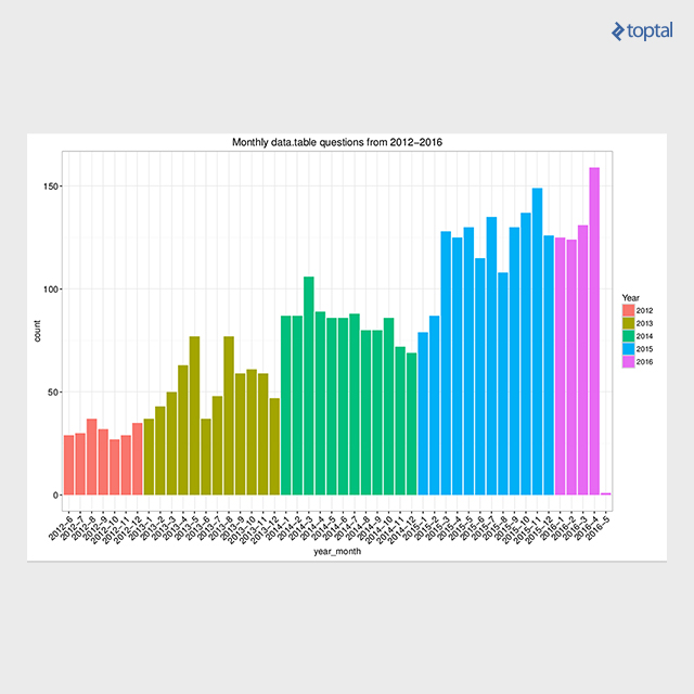
Ample resources are available, including function manuals and package vignettes offering subject-specific tutorials. These resources can be found on the Getting started page. The Presentations page lists over 30 materials (slides, videos, etc.) from data.table presentations worldwide. Additionally, a thriving community provides support, with over 4,000 questions tagged with data.table on Stack Overflow, boasting a high answer rate (91.9%). The plot below depicts the trend of data.table tagged questions on Stack Overflow over time.

SO questions monthly for data.table - Only data.table tagged questions, not ones with data.table (accepted) answers

Conclusion

This article presents select examples for efficient tabular data transformation in R using the data.table package. For concrete performance figures, refer to reproducible benchmarks. My blog post, Solve common R problems efficiently with data.table, summarizes data.table solutions for the top 50 rated Stack Overflow questions related to the R language, providing numerous figures and reproducible code. The data.table package employs native implementations of fast radix ordering for grouping and binary search for efficient subsets/joins. Radix ordering was incorporated into base R from version 3.3.0 onwards. Recently, this algorithm was implemented and parallelized within the H2O machine learning platform for use across H2O clusters, further enhancing its capabilities enabling efficient big joins on 10B x 10B rows.

Licensed under CC BY-NC-SA 4.0