Scala has become increasingly popular in recent years due to its seamless blend of functional and object-oriented programming paradigms, and its execution on the reliable Java Virtual Machine (JVM).

Despite compiling to Java bytecode, Scala is crafted to address several limitations perceived in Java. Offering comprehensive functional programming support, Scala’s syntax incorporates many implicit constructs that Java developers must build manually, often with significant complexity.

Developing a language that compiles to Java bytecode necessitates a profound understanding of the JVM’s internal mechanisms. To grasp the achievements of Scala’s creators, it’s crucial to delve deeper and examine how the compiler translates Scala source code into efficient JVM bytecode.

Let’s explore how these aspects are implemented.

Prerequisites

This article assumes a fundamental understanding of Java Virtual Machine bytecode. The complete virtual machine specification is available from Oracle’s official documentation. However, reading the entire specification isn’t essential for comprehending this article. I’ve provided a concise guide at the end for a quick introduction.

You’ll need a tool to disassemble Java bytecode to replicate the provided examples and conduct further investigation. The Java Development Kit includes a command-line utility called javap, which we’ll utilize here. A brief demonstration of javap is included in the guide at the end.

Naturally, readers who wish to follow along with the examples will require a functional installation of the Scala compiler. This article was written using Scala 2.11.7. Different Scala versions might generate slightly different bytecode.

Default Getters and Setters

While Java conventions dictate providing getter and setter methods for public attributes, Java programmers must write them explicitly, even though the pattern has remained unchanged for decades. In contrast, Scala offers default getters and setters.

Consider the following example:

1
2

class Person(val name:String) {
}

Let’s examine the Person class. Compiling this file with scalac and then executing $ javap -p Person.class yields:

1
2
3
4
5
6

Compiled from "Person.scala"
public class Person {
  private final java.lang.String name;   // field
  public java.lang.String name();        // getter method
  public Person(java.lang.String);       // constructor
}

As evident, for every field in the Scala class, a corresponding field and getter method are generated. The field is private and final, while the method is public.

If we modify the Person source code by replacing val with var and recompile, the field’s final modifier is removed, and the setter method is also included:

1
2
3
4
5
6
7

Compiled from "Person.scala"
public class Person {
  private java.lang.String name;            // field
  public java.lang.String name();           // getter method
  public void name_$eq(java.lang.String);   // setter method
  public Person(java.lang.String);          // constructor
}

When a val or var is defined within the class body, the corresponding private field and accessor methods are created and initialized accordingly during instance creation.

It’s worth noting that this implementation of class-level val and var fields implies that if any variables are used at the class level to store temporary values and are never accessed directly by the programmer, initializing each such field will add one or two methods to the class footprint. Adding a private modifier to such fields doesn’t eliminate the corresponding accessors; it merely makes them private.

Variable and Function Definitions

Suppose we have a method called m() and create three different Scala-style references to this function:

 1
 2
 3
 4
 5
 6
 7
 8
 9
10

class Person(val name:String) {
    def m(): Int = {
      // ...
      return 0
    }

    val m1 = m
    var m2 = m
    def m3 = m
}

How are these references to m constructed? When is m executed in each case? Let’s analyze the resulting bytecode. The following output displays the results of javap -v Person.class (excluding extraneous output):

 1
 2
 3
 4
 5
 6
 7
 8
 9
10
11
12
13
14
15
16
17
18
19
20
21
22
23
24
25
26
27
28
29
30
31
32
33
34
35
36
37
38
39
40
41
42
43
44
45
46
47
48
49
50
51
52
53
54
55
56
57
58
59
60
61

Constant pool:
  #22 = Fieldref           #2.#21         // Person.m1:I
  #24 = Fieldref           #2.#23         // Person.m2:I
  #30 = Methodref          #2.#29         // Person.m:()I
  #35 = Methodref          #4.#34         // java/lang/Object."<init>":()V

  // ...

  public int m();
    Code:
         // other methods refer to this method
         // ...

  public int m1();
    Code:
         // get the value of field m1 and return it
         0: aload_0
         1: getfield      #22                 // Field m1:I
         4: ireturn

  public int m2();
    Code:
         // get the value of field m2 and return it
         0: aload_0
         1: getfield      #24                 // Field m2:I
         4: ireturn

  public void m2_$eq(int);
    Code:
         // get the value of this method's input argument
         0: aload_0
         1: iload_1

         // write it to the field m2 and return
         2: putfield      #24                 // Field m2:I
         5: return

  public int m3();
    Code:
         // execute the instance method m(), and return
         0: aload_0
         1: invokevirtual #30                 // Method m:()I
         4: ireturn

  public Person(java.lang.String);
    Code:
        // instance constructor ...

        // execute the instance method m(), and write the result to field m1
         9: aload_0
        10: aload_0
        11: invokevirtual #30                 // Method m:()I
        14: putfield      #22                 // Field m1:I

        // execute the instance method m(), and write the result to field m2
        17: aload_0
        18: aload_0
        19: invokevirtual #30                 // Method m:()I
        22: putfield      #24                 // Field m2:I

        25: return   

The constant pool reveals that the reference to method m() is stored at index #30. Examining the constructor code, we observe that this method is invoked twice during initialization, with the instruction invokevirtual #30 appearing initially at byte offset 11 and then at offset 19. The first invocation is followed by the instruction putfield #22, which assigns the method’s result to the field m1, referenced by index #22 in the constant pool. The second invocation follows the same pattern, assigning the value to the field m2, indexed at #24 in the constant pool.

In essence, assigning a method to a variable declared with val or var only assigns the result of the method to that variable. We can see that the generated methods m1() and m2() are simply getters for these variables. In the case of var m2, we also observe the creation of the setter m2_$eq(int), which behaves like any other setter, overwriting the field’s value.

However, employing the keyword def produces a different outcome. Instead of retrieving a field value to return, the method m3() also includes the instruction invokevirtual #30. This means that whenever this method is called, it subsequently calls m() and returns the result of that method.

Therefore, Scala offers three ways to work with class fields, easily specified using the keywords val, var, and def. In Java, we would need to implement the necessary setters and getters explicitly, resulting in less expressive and more error-prone boilerplate code.

Lazy Values

The generated code becomes more intricate when declaring a lazy value. Let’s assume we add the following field to the previously defined class:

1

lazy val m4 = m

Running javap -p -v Person.class now reveals the following:

 1
 2
 3
 4
 5
 6
 7
 8
 9
10
11
12
13
14
15
16
17
18
19
20
21
22
23
24
25
26
27
28
29
30
31
32
33
34
35
36
37
38
39
40
41
42
43
44
45
46
47
48
49
50
51
52
53
54
55
56
57
58
59
60
61
62
63
64
65
66
67
68
69
70
71
72

Constant pool:
  #20 = Fieldref           #2.#19         // Person.bitmap$0:Z
  #23 = Methodref          #2.#22         // Person.m:()I
  #25 = Fieldref           #2.#24         // Person.m4:I
  #31 = Fieldref           #27.#30        // scala/runtime/BoxedUnit.UNIT:Lscala/runtime/BoxedUnit;
  #48 = Methodref          #2.#47         // Person.m4$lzycompute:()I

  // ...

  private volatile boolean bitmap$0;

  private int m4$lzycompute();
    Code:
        // lock the thread
         0: aload_0
         1: dup
         2: astore_1
         3: monitorenter

        // check the flag for whether this field has already been set
         4: aload_0
         5: getfield      #20                 // Field bitmap$0:Z

        // if it has, skip to position 24 (unlock the thread and return)
         8: ifne          24

        // if it hasn't, execute the method m()
        11: aload_0
        12: aload_0
        13: invokevirtual #23                 // Method m:()I

        // write the method to the field m4
        16: putfield      #25                 // Field m4:I

        // set the flag indicating the field has been set
        19: aload_0
        20: iconst_1
        21: putfield      #20                 // Field bitmap$0:Z

        // unlock the thread
        24: getstatic     #31                 // Field scala/runtime/BoxedUnit.UNIT:Lscala/runtime/BoxedUnit;
        27: pop
        28: aload_1
        29: monitorexit

        // get the value of field m4 and return it
        30: aload_0
        31: getfield      #25                 // Field m4:I
        34: ireturn

        // ...

  public int m4();
    Code:
        // check the flag for whether this field has already been set
         0: aload_0
         1: getfield      #20                 // Field bitmap$0:Z

        // if it hasn't, skip to position 14 (invoke lazy method and return)
         4: ifeq          14

        // if it has, get the value of field m4, then skip to position 18 (return)
         7: aload_0
         8: getfield      #25                 // Field m4:I
        11: goto          18

        // execute the method m4$lzycompute() to set the field
        14: aload_0
        15: invokespecial #48                 // Method m4$lzycompute:()I

        // return
        18: ireturn

In this scenario, the value of the field m4 is not computed until required. The compiler generates a special private method called m4$lzycompute() to calculate the lazy value and the field bitmap$0 to monitor its state. The method m4() checks if the field’s value is 0, signifying that m4 has not been initialized. If so, it invokes m4$lzycompute(), populates m4, and returns its value. This private method also sets the value of bitmap$0 to 1, ensuring that the next time m4() is called, it bypasses the initialization method and directly returns the value of m4.

Scala generates bytecode that is both thread-safe and efficient. To achieve thread safety, the lazy compute method utilizes the monitorenter/monitorexit instruction pair. Efficiency is maintained because the synchronization overhead only occurs during the first read of the lazy value.

A single bit is sufficient to indicate the state of the lazy value. Consequently, a single int field can track up to 32 lazy values. If the source code defines more than one lazy value, the compiler modifies the bytecode to implement a bitmask for this purpose.

Once again, Scala allows us to leverage a specific behavior that would require explicit implementation in Java, saving effort and minimizing the potential for errors.

Function as Value

Let’s now examine the following Scala source code:

1
2
3
4
5
6
7
8
9

class Printer(val output: String => Unit) {
}

object Hello {
    def main(arg: Array[String]) {
        val printer = new Printer( s => println(s) );
        printer.output("Hello");
    }
}

The Printer class has a field named output with the type String => Unit, representing a function that takes a String and returns an object of type Unit (similar to void in Java). In the main method, we create an instance of this object and assign an anonymous function to the field that prints a given string.

Compiling this code generates four class files:

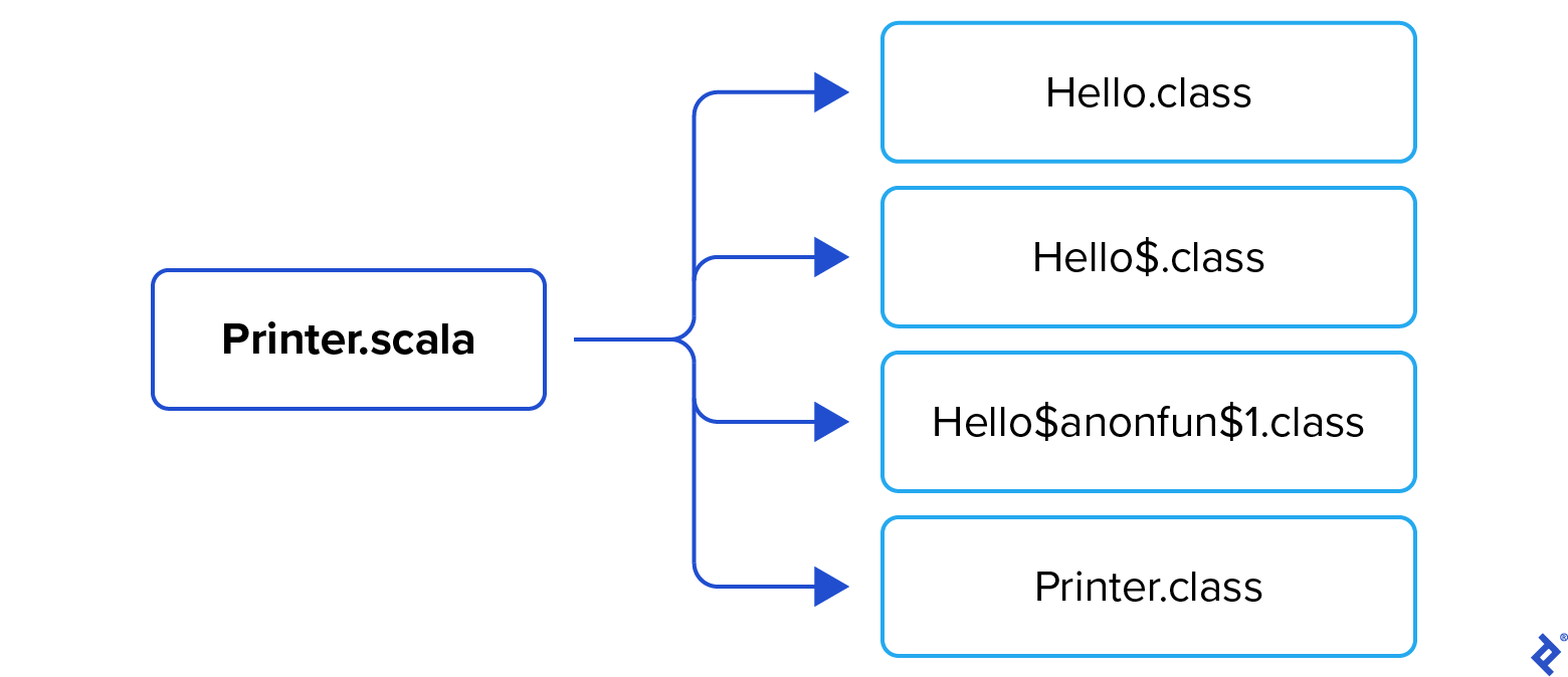
Hello.class acts as a wrapper class whose main method simply invokes Hello$.main():

 1
 2
 3
 4
 5
 6
 7
 8
 9
10

public final class Hello

  // ...

  public static void main(java.lang.String[]);
    Code:
         0: getstatic     #16                 // Field Hello$.MODULE$:LHello$;
         3: aload_0
         4: invokevirtual #18                 // Method Hello$.main:([Ljava/lang/String;)V
         7: return

The hidden Hello$.class houses the actual implementation of the main method. To examine its bytecode, ensure you properly escape the $ character according to your command shell’s rules to prevent its interpretation as a special character:

 1
 2
 3
 4
 5
 6
 7
 8
 9
10
11
12
13
14
15
16
17
18
19
20
21
22
23
24
25
26

public final class Hello$

// ...

  public void main(java.lang.String[]);
    Code:
         // initialize Printer and anonymous function
         0: new           #16                 // class Printer
         3: dup
         4: new           #18                 // class Hello$anonfun$1
         7: dup
         8: invokespecial #19                 // Method Hello$anonfun$1."<init>":()V
        11: invokespecial #22                 // Method Printer."<init>":(Lscala/Function1;)V
        14: astore_2

        // load the anonymous function onto the stack
        15: aload_2
        16: invokevirtual #26                 // Method Printer.output:()Lscala/Function1;

        // execute the anonymous function, passing the string "Hello"
        19: ldc           #28                 // String Hello
        21: invokeinterface #34,  2           // InterfaceMethod scala/Function1.apply:(Ljava/lang/Object;)Ljava/lang/Object;

        // return
        26: pop
        27: return

The method instantiates a Printer object and creates a Hello$$anonfun$1 object containing our anonymous function s => println(s). The Printer is initialized with this object as the value for the output field. This field is then loaded onto the stack and executed with the operand "Hello".

Next, let’s analyze the anonymous function class, Hello$$anonfun$1.class. We can observe that it extends Scala’s Function1 (as AbstractFunction1) by implementing the apply() method. It actually creates two apply() methods, one wrapping the other, responsible for type checking (in this case, ensuring the input is a String) and executing the anonymous function (printing the input using println()).

 1
 2
 3
 4
 5
 6
 7
 8
 9
10
11
12
13
14
15
16
17
18
19
20
21
22
23
24
25
26
27
28
29

public final class Hello$anonfun$1 extends scala.runtime.AbstractFunction1<java.lang.String, scala.runtime.BoxedUnit> implements scala.Serializable

  // ...

  // Takes an argument of type String. Invoked second.
  public final void apply(java.lang.String);
    Code:
        // execute Scala's built-in method println(), passing the input argument
         0: getstatic     #25                 // Field scala/Predef$.MODULE$:Lscala/Predef$;
         3: aload_1
         4: invokevirtual #29                 // Method scala/Predef$.println:(Ljava/lang/Object;)V

         7: return

  // Takes an argument of type Object. Invoked first.
  public final java.lang.Object apply(java.lang.Object);
    Code:
         0: aload_0

        // check that the input argument is a String (throws exception if not)
         1: aload_1
         2: checkcast     #36                 // class java/lang/String

        // invoke the method apply( String ), passing the input argument
         5: invokevirtual #38                 // Method apply:(Ljava/lang/String;)V

        // return the void type
         8: getstatic     #44                 // Field scala/runtime/BoxedUnit.UNIT:Lscala/runtime/BoxedUnit;
        11: areturn

Referring back to the Hello$.main() method above, we see that at offset 21, the anonymous function is invoked by calling its apply( Object ) method.

Lastly, for completeness, let’s examine the bytecode for Printer.class:

 1
 2
 3
 4
 5
 6
 7
 8
 9
10
11
12
13
14
15
16
17
18
19
20
21
22
23

public class Printer

  // ...

  // field
  private final scala.Function1<java.lang.String, scala.runtime.BoxedUnit> output;

  // field getter
  public scala.Function1<java.lang.String, scala.runtime.BoxedUnit> output();
    Code:
         0: aload_0
         1: getfield      #14                 // Field output:Lscala/Function1;
         4: areturn

  // constructor
  public Printer(scala.Function1<java.lang.String, scala.runtime.BoxedUnit>);
    Code:
         0: aload_0
         1: aload_1
         2: putfield      #14                 // Field output:Lscala/Function1;
         5: aload_0
         6: invokespecial #21                 // Method java/lang/Object."<init>":()V
         9: return

The anonymous function is treated like any other val variable, stored in the class field output, and the getter method output() is generated. The only distinction is that this variable must now implement the Scala interface scala.Function1 (which AbstractFunction1 does).

Therefore, the cost of this elegant Scala feature is the underlying utility classes created to represent and execute a single anonymous function that can be used as a value. You should consider the number of such functions and your VM implementation’s details to determine the implications for your application.

Scala Traits

Scala traits resemble interfaces in Java. The following trait defines two method signatures and provides a default implementation for the second one. Let’s see how it’s implemented:

1
2
3
4

trait Similarity {
  def isSimilar(x: Any): Boolean
  def isNotSimilar(x: Any): Boolean = !isSimilar(x)
}

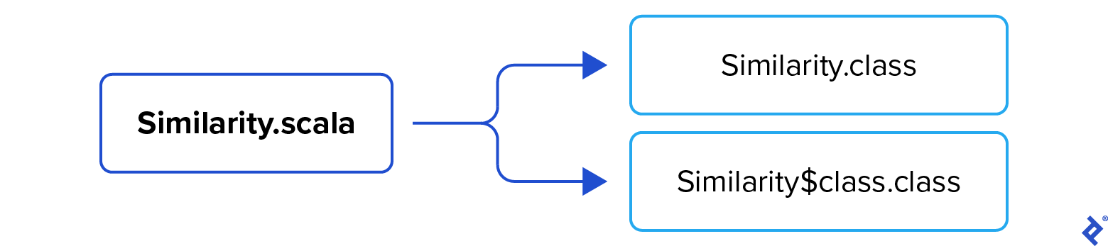
Two entities are generated: Similarity.class, the interface declaring both methods, and the synthetic class Similarity$class.class, which provides the default implementation:

1
2
3
4

public interface Similarity {
  public abstract boolean isSimilar(java.lang.Object);
  public abstract boolean isNotSimilar(java.lang.Object);
}

 1
 2
 3
 4
 5
 6
 7
 8
 9
10
11
12
13
14
15
16
17
18
19
20
21
22
23
24

public abstract class Similarity$class

  public static boolean isNotSimilar(Similarity, java.lang.Object);
    Code:
         0: aload_0

        // execute the instance method isSimilar()
         1: aload_1
         2: invokeinterface #13,  2           // InterfaceMethod Similarity.isSimilar:(Ljava/lang/Object;)Z

        // if the returned value is 0, skip to position 14 (return with value 1)
         7: ifeq          14

        // otherwise, return with value 0
        10: iconst_0
        11: goto          15

        // return the value 1
        14: iconst_1
        15: ireturn

  public static void $init$(Similarity);
    Code:
         0: return

When a class implements this trait and calls the isNotSimilar method, the Scala compiler generates the bytecode instruction invokestatic to call the static method provided by the accompanying class.

Traits can be combined to create intricate polymorphism and inheritance structures. For instance, multiple traits and the implementing class can all override a method with the same signature, using super.methodName() to delegate control to the next trait. When the Scala compiler encounters such calls:

• It identifies the specific trait assumed by the call.
• It determines the name of the accompanying class that provides the static method bytecode defined for the trait.
• It generates the necessary invokestatic instruction.

Hence, the powerful concept of traits is implemented at the JVM level without incurring significant overhead, allowing Scala programmers to utilize this feature without concerns about runtime performance.

Singletons

Scala allows the explicit definition of singleton classes using the object keyword. Consider the following singleton class:

1
2
3

object Config {
   val home_dir = "/home/user"
}

The compiler produces two class files:

Config.class is relatively straightforward:

1
2
3
4
5
6
7
8

public final class Config

  public static java.lang.String home_dir();
    Code:
      // execute the method Config$.home_dir()
       0: getstatic     #16                 // Field Config$.MODULE$:LConfig$;
       3: invokevirtual #18                 // Method Config$.home_dir:()Ljava/lang/String;
       6: areturn

It serves as a decorator for the synthetic Config$ class, which encapsulates the singleton’s functionality. Examining this class with javap -p -c reveals the following bytecode:

 1
 2
 3
 4
 5
 6
 7
 8
 9
10
11
12
13
14
15
16
17
18
19
20
21
22
23
24
25
26
27
28
29
30
31
32
33
34
35
36

public final class Config$

  public static final Config$ MODULE$;        // a public reference to the singleton object

  private final java.lang.String home_dir;

  // static initializer
  public static {};
    Code:
         0: new           #2                  // class Config$
         3: invokespecial #12                 // Method "<init>":()V
         6: return

  public java.lang.String home_dir();
    Code:
        // get the value of field home_dir and return it
         0: aload_0
         1: getfield      #17                 // Field home_dir:Ljava/lang/String;
         4: areturn

  private Config$();
    Code:
        // initialize the object
         0: aload_0
         1: invokespecial #19                 // Method java/lang/Object."<init>":()V

        // expose a public reference to this object in the synthetic variable MODULE$
         4: aload_0
         5: putstatic     #21                 // Field MODULE$:LConfig$;

        // load the value "/home/user" and write it to the field home_dir
         8: aload_0
         9: ldc           #23                 // String /home/user
        11: putfield      #17                 // Field home_dir:Ljava/lang/String;

        14: return

It consists of the following:

• The synthetic variable MODULE$, providing access to the singleton object.
• The static initializer {} (also known as <clinit>, the class initializer) and the private method Config$, responsible for initializing MODULE$ and setting its fields to default values.
• A getter method for the static field home_dir. In this case, there’s only one method. If the singleton has more fields, it will have additional getters and setters for mutable fields.

The singleton pattern is a widely used and valuable design pattern. While Java doesn’t offer a direct language-level mechanism for specifying singletons, Scala provides a clear and convenient way to declare them explicitly using the object keyword. As we’ve observed, its implementation is both efficient and straightforward.

Conclusion

We’ve explored how Scala compiles several implicit and functional programming features into sophisticated Java bytecode structures. This glimpse into Scala’s inner workings provides a deeper appreciation for its capabilities, enabling us to maximize its potential.

Moreover, we now possess the tools to investigate the language independently. Numerous other useful features of Scala’s syntax, such as case classes, currying, and list comprehensions, are beyond the scope of this article. I encourage you to delve into Scala’s implementation of these constructs and become a true Scala ninja!

The Java Virtual Machine: A Crash Course

Similar to the Java compiler, the Scala compiler transforms source code into .class files containing Java bytecode for execution by the Java Virtual Machine. To comprehend the differences between the two languages under the hood, it’s essential to understand their target system. This section provides a concise overview of crucial elements in the Java Virtual Machine architecture, class file structure, and assembler fundamentals.

This guide only covers the minimum necessary to follow the article’s content. While many significant JVM components are omitted here, comprehensive information is available in the official documentation: here.

Decompiling Class Files with javap Constant Pool Field and Method Tables JVM Bytecode Method Calls and the Call Stack Execution on the Operand Stack Local Variables Return to Top

Decompiling Class Files with javap

Java includes the command-line utility javap, which decompiles .class files into a human-readable format. Since both Scala and Java class files target the same JVM, javap can be used to inspect class files compiled from Scala code.

Let’s compile the following source code:

1
2
3
4
5
6
7
8

// RegularPolygon.scala
class RegularPolygon( val numSides: Int ) {

  def getPerimeter( sideLength: Double ): Double = {
    println( "Calculating perimeter..." )
    return sideLength * this.numSides
  }
}

Compiling with scalac RegularPolygon.scala generates RegularPolygon.class. Executing javap RegularPolygon.class displays the following output:

1
2
3
4
5
6
7

$ javap RegularPolygon.class
Compiled from "RegularPolygon.scala"
public class RegularPolygon {
  public int numSides();
  public double getPerimeter(double);
  public RegularPolygon(int);
}

This is a basic breakdown of the class file, showing the names and types of the class’s public members. Adding the -p option includes private members:

1
2
3
4
5
6
7
8

$ javap -p RegularPolygon.class
Compiled from "RegularPolygon.scala"
public class RegularPolygon {
  private final int numSides;
  public int numSides();
  public double getPerimeter(double);
  public RegularPolygon(int);
}

This still doesn’t provide much information. To examine the implementation of methods in Java bytecode, let’s use the -c option:

 1
 2
 3
 4
 5
 6
 7
 8
 9
10
11
12
13
14
15
16
17
18
19
20
21
22
23
24
25
26
27
28
29
30
31
32

$ javap -p -c RegularPolygon.class
Compiled from "RegularPolygon.scala"
public class RegularPolygon {
  private final int numSides;

  public int numSides();
    Code:
       0: aload_0
       1: getfield      #13                 // Field numSides:I
       4: ireturn

  public double getPerimeter(double);
    Code:
       0: getstatic     #23                 // Field scala/Predef$.MODULE$:Lscala/Predef$;
       3: ldc           #25                 // String Calculating perimeter...
       5: invokevirtual #29                 // Method scala/Predef$.println:(Ljava/lang/Object;)V
       8: dload_1
       9: aload_0
      10: invokevirtual #31                 // Method numSides:()I
      13: i2d
      14: dmul
      15: dreturn

  public RegularPolygon(int);
    Code:
       0: aload_0
       1: iload_1
       2: putfield      #13                 // Field numSides:I
       5: aload_0
       6: invokespecial #38                 // Method java/lang/Object."<init>":()V
       9: return
}

This is more interesting, but to get the complete picture, we’ll use the -v or -verbose option, as in javap -p -v RegularPolygon.class:

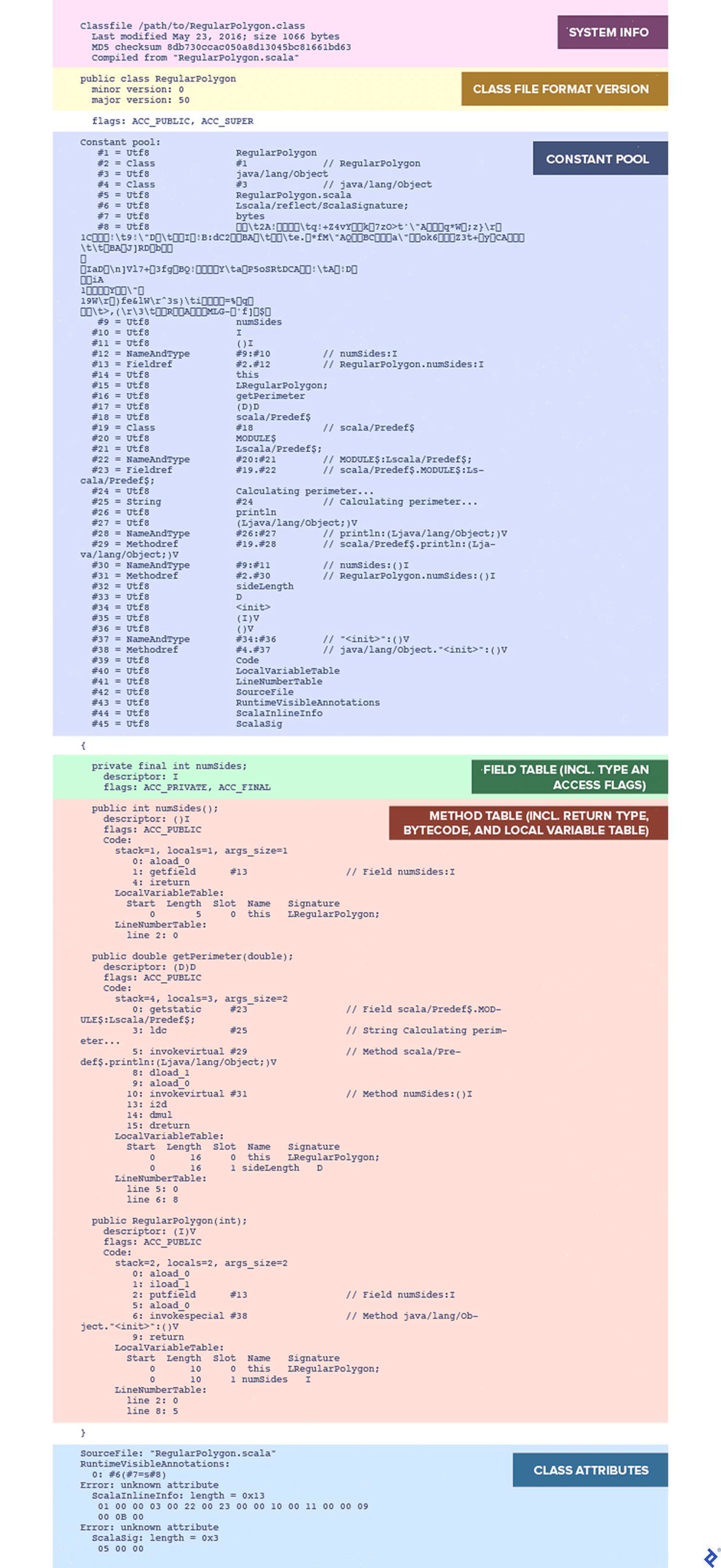
Now we see the class file’s contents. Let’s break down some crucial parts.

Constant Pool

The C++ development cycle involves compilation and linking stages. However, Java skips an explicit linking stage because linking occurs at runtime. The class file must support this runtime linking, meaning that when source code references any field or method, the resulting bytecode must retain relevant references in symbolic form. These symbolic references are resolved by the runtime linker once the application loads into memory and actual addresses become available. This symbolic form must contain:

• class name
• field or method name
• type information

The class file format specification includes a section called the constant pool, a table of all references required by the linker. It consists of entries with various types.

1
2
3
4
5
6
7

// ...
Constant pool:
   #1 = Utf8               RegularPolygon
   #2 = Class              #1             // RegularPolygon
   #3 = Utf8               java/lang/Object
   #4 = Class              #3             // java/lang/Object
   // ...

The first byte of each entry is a numeric tag identifying the entry type. The remaining bytes provide information about the entry’s value, with the number of bytes and interpretation rules depending on the type indicated by the first byte.

For instance, a Java class using the constant integer 365 might have a constant pool entry with the following bytecode:

1

x03 00 00 01 6D

The first byte, x03, identifies the entry type as CONSTANT_Integer, informing the linker that the next four bytes represent the integer’s value. (Note that 365 in hexadecimal is x16D.) If this is the 14th entry in the constant pool, javap -v displays it as:

1

#14 = Integer            365

Many constant types are composed of references to more “primitive” constant types elsewhere in the constant pool. For example, our sample code includes the statement:

1

println( "Calculating perimeter..." )

Using a string constant results in two constant pool entries: one with type CONSTANT_String and another with type CONSTANT_Utf8. The Constant_UTF8 entry contains the actual UTF8 representation of the string value, while the CONSTANT_String entry references the CONSTANT_Utf8 entry:

1
2

#24 = Utf8               Calculating perimeter...
#25 = String             #24            // Calculating perimeter...

This complexity arises because other constant pool entry types reference Utf8 entries but are not String entries themselves. For instance, any reference to a class attribute generates a CONSTANT_Fieldref entry, which contains references to the class name, attribute name, and attribute type:

1
2
3
4
5
6

 #1 = Utf8               RegularPolygon
 #2 = Class              #1             // RegularPolygon
 #9 = Utf8               numSides
#10 = Utf8               I
#12 = NameAndType        #9:#10         // numSides:I
#13 = Fieldref           #2.#12         // RegularPolygon.numSides:I

For a more detailed explanation of the constant pool, refer to the JVM documentation.

Field and Method Tables

Each class file contains a field table with information about every field (attribute) defined in the class. These are references to constant pool entries describing the field’s name, type, access control flags, and other relevant data.

A similar method table is also present in the class file. However, besides name and type information, it contains the actual bytecode instructions executed by the JVM for each non-abstract method, along with data structures used by the method’s stack frame (described later).

JVM Bytecode

The JVM employs its internal instruction set to execute compiled code. Running javap with the -c option displays the compiled method implementations. Inspecting our RegularPolygon.class file this way, we see the following output for the getPerimeter() method:

 1
 2
 3
 4
 5
 6
 7
 8
 9
10
11

public double getPerimeter(double);
  Code:
     0: getstatic     #23                 // Field scala/Predef$.MODULE$:Lscala/Predef$;
     3: ldc           #25                 // String Calculating perimeter...
     5: invokevirtual #29                 // Method scala/Predef$.println:(Ljava/lang/Object;)V
     8: dload_1
     9: aload_0
    10: invokevirtual #31                 // Method numSides:()I
    13: i2d
    14: dmul
    15: dreturn

The actual bytecode might resemble:

1
2
3
4
5

xB2 00 17
x12 19
xB6 00 1D
x27
...

Each instruction begins with a one-byte opcode identifying the JVM instruction, followed by zero or more instruction operands depending on the specific instruction’s format. These operands are typically constant values or references to the constant pool. javap helpfully translates the bytecode into a human-readable form, displaying:

• The offset, representing the instruction’s first byte’s position within the code.
• The human-readable name or mnemonic of the instruction.
• The operand’s value, if any.

Operands displayed with a pound sign, such as #23, are references to constant pool entries. As shown, javap also generates helpful comments identifying the referenced pool entry.

We’ll discuss some common instructions below. For comprehensive information about the complete JVM instruction set, refer to the documentation.

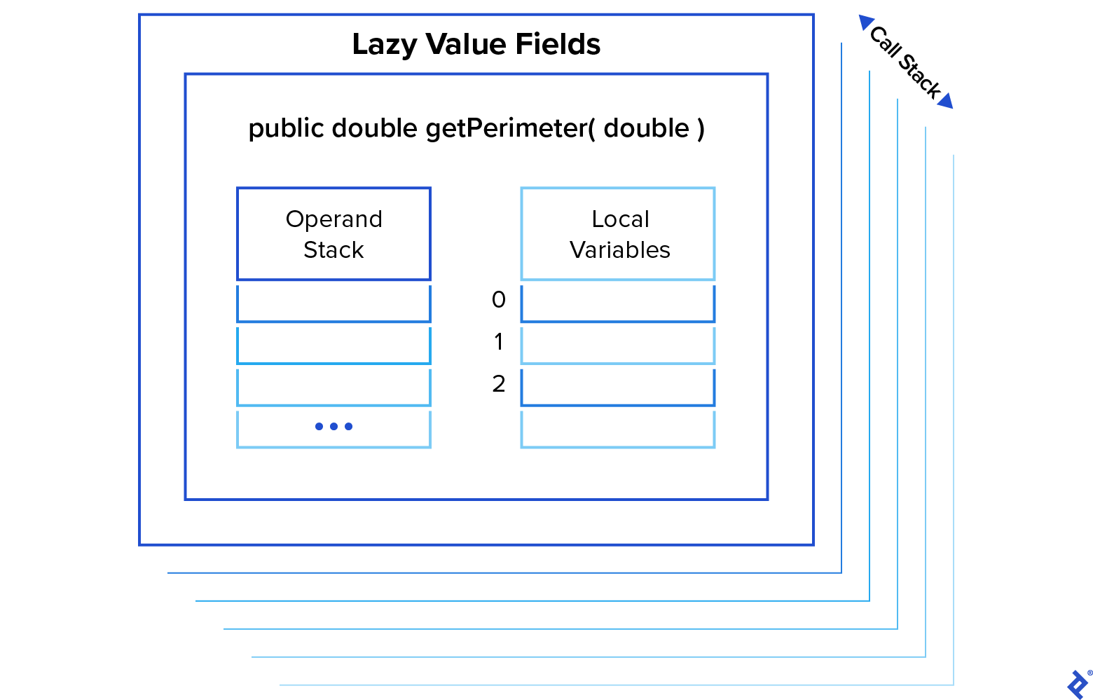
Method Calls and the Call Stack

Each method call requires its own execution context, including locally declared variables and arguments passed to the method. Together, these constitute a stack frame. Upon method invocation, a new frame is created and placed on top of the call stack. When the method returns, the current frame is removed and discarded, restoring the frame that was active before the method call.

A stack frame comprises several distinct structures. Two crucial ones are the operand stack and the local variable table, discussed next.

Execution on the Operand Stack

Many JVM instructions operate on their frame’s operand stack. Instead of explicitly specifying a constant operand in the bytecode, these instructions take values from the operand stack’s top as input, typically removing these values during the process. Some instructions also push new values onto the stack. This way, JVM instructions can be combined to perform complex operations. For example, the expression:

1

sideLength * this.numSides

compiles to the following in our getPerimeter() method:

1
2
3
4
5

 8: dload_1
 9: aload_0
10: invokevirtual #31                 // Method numSides:()I
13: i2d
14: dmul

• The first instruction, dload_1, pushes the object reference from slot 1 of the local variable table (discussed next) onto the operand stack. In this case, it’s the method argument sideLength.
• Next, aload_0 pushes the object reference at slot 0 of the local variable table onto the operand stack. This is almost always the reference to this, the current class.
• This sets up the stack for the subsequent call, invokevirtual #31, which executes the instance method numSides(). invokevirtual pops the top operand (the reference to this) to determine the class from which to call the method. Upon method return, its result is pushed onto the stack.
• Here, the returned value (numSides) is an integer. It needs conversion to a double floating-point format for multiplication with another double value. The instruction i2d pops the integer value, converts it to floating-point format, and pushes it back onto the stack.
• At this point, the stack contains the floating-point result of this.numSides on top, followed by the value of the sideLength argument passed to the method. dmul pops these two values, performs floating-point multiplication, and pushes the result onto the stack.

When a method is called, a new operand stack is created as part of its stack frame, where operations are performed. It’s important to distinguish between the terms “stack,” which can refer to the call stack (the stack of frames providing context for method execution) or a specific frame’s operand stack (where JVM instructions operate).

Local Variables

Each stack frame maintains a table of local variables, typically including a reference to the this object, arguments passed during the method call, and any local variables declared within the method body. Running javap with the -v option displays information about setting up each method’s stack frame, including its local variable table:

 1
 2
 3
 4
 5
 6
 7
 8
 9
10
11
12
13
14

public double getPerimeter(double);

// ...

Code:
     0: getstatic     #23                 // Field scala/Predef$.MODULE$:Lscala/Predef$;
     3: ldc           #25                 // String Calculating perimeter...

     // ...

  LocalVariableTable:
    Start  Length  Slot  Name   Signature
        0      16     0  this   LRegularPolygon;
        0      16     1 sideLength   D

In this example, there are two local variables. The variable in slot 0 is named this and has the type RegularPolygon, representing the reference to the method’s own class. The variable in slot 1 is named sideLength and has the type D (indicating a double), representing the argument passed to our getPerimeter() method.

Instructions such as iload_1, fstore_2, or aload [n] transfer different types of local variables between the operand stack and the local variable table. Since the first item in the table is usually the reference to this, the instruction aload_0 is common in methods operating on their own class.

This concludes our brief exploration of JVM basics.