The Protein Data Bank (PDB) serves as a central resource for experimentally-determined structures of proteins, nucleic acids, and complex assemblies. All the data housed in the PDB is obtained through experimental techniques such as X-ray crystallography, spectroscopy, NMR, and other methods.

This article outlines a methodology for extracting, filtering, and cleaning data from the PDB, ultimately facilitating the kind of analysis detailed in the article Occurrence of protein disulfide bonds in different domains of life: a comparison of proteins from the Protein Data Bank, featured in Protein Engineering, Design and Selection, Volume 27, Issue 3, 1 March 2014, pp. 65–72.

The PDB often includes numerous repeating structures with variations in resolution, methodologies, mutations, and other factors. Conducting experiments with identical or highly similar proteins can introduce bias into group analysis. To address this, we need to carefully select an appropriate structure from a set of duplicates, necessitating the use of a non-redundant (NR) set of proteins.

For normalization purposes, I suggest downloading the chemical compound dictionary for importing atom names into a database that uses 3NF or uses a star schema and dimensional modeling. (I’ve also used DSSP to aid in the removal of problematic structures. While I won’t delve into the details in this article, it’s worth noting that I haven’t utilized any other DSSP features.)

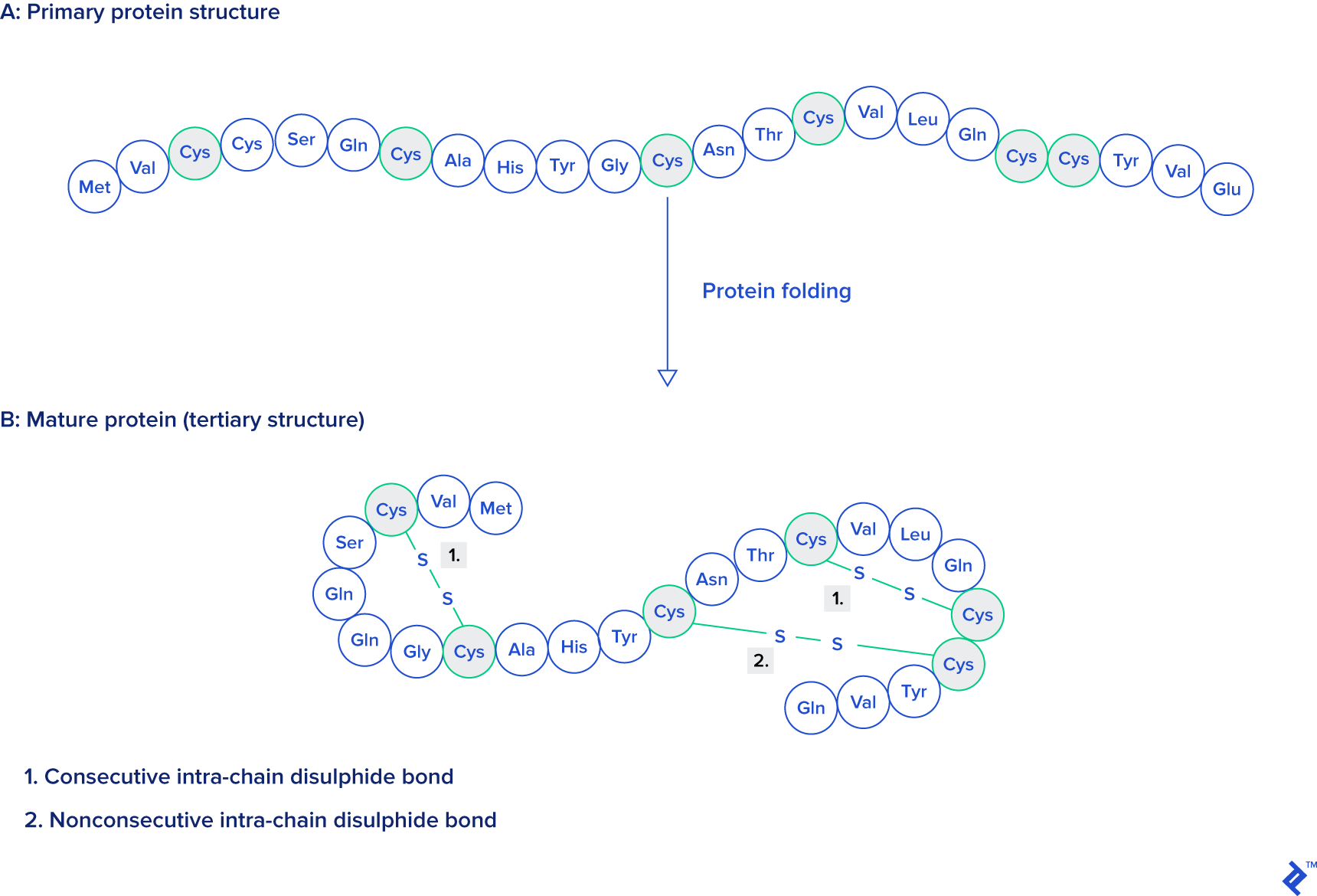
The data employed in this study comprises single-unit proteins from various species that contain at least one disulfide bond. For analysis, all disulfide bonds are categorized as consecutive or nonconsecutive, categorized by domain (archaea, prokaryote, viral, eukaryote, or other), and classified by length.

Output

To facilitate analysis in tools like R or SPSS, the data needs to be structured in a database table as follows:

Materials and Methods

To achieve this objective, the first step involves gathering data from rcsb.org, a repository offering downloadable PDB structures of experiments in various formats.

While data is stored in multiple formats, this example will focus on the formatted fixed-space delimited textual format (PDB). An alternative to the PDB textual format is PDBML, its XML counterpart, but it occasionally exhibits issues with malformed atom position naming entries, potentially hindering data analysis. Although older formats like mmCIF might be accessible, they won’t be covered in this article.

The PDB Format

The PDB format utilizes a fragmented fixed-width textual format, easily parsed by SQL queries, Java plugins, or Perl modules, for instance. Each data type within the file container is represented by a line commencing with the corresponding tag—we will explore each tag type in the subsequent subsections. The line length is capped at 80 characters, with tags occupying a maximum of six characters plus one or more spaces, collectively consuming eight bytes. However, there are instances where spaces are omitted between tags and data, typically for CONECT tags.

TITLE

The TITLE tag designates a line as part of the experiment’s title, encompassing the molecule name and other pertinent information like the insertion, mutation, or deletion of a specific amino acid.

1
2
3
4

12345678901234567890123456789012345678901234567890123456789012345678901234567890
TITLE     A TWO DISULFIDE DERIVATIVE OF CHARYBDOTOXIN WITH DISULFIDE            
TITLE    2 13-33 REPLACED BY TWO ALPHA-AMINOBUTYRIC ACIDS, NMR, 30              
TITLE    3 STRUCTURES                                                           

When a TITLE record spans multiple lines, the title needs to be concatenated based on a continuation number, right-aligned on bytes 9 and 10 (depending on the number of lines).

ATOM

ATOM lines contain coordinate data for each atom in an experiment. Due to insertions, mutations, alternate locations, or multiple models within an experiment, the same atom might be repeated multiple times. The process of selecting the correct atoms will be explained later.

1
2
3
4
5
6
7
8

12345678901234567890123456789012345678901234567890123456789012345678901234567890
ATOM    390  N   GLY A  26      -1.120  -2.842   4.624  1.00  0.00           N  
ATOM    391  CA  GLY A  26      -0.334  -2.509   3.469  1.00  0.00           C  
ATOM    392  C   GLY A  26       0.682  -1.548   3.972  1.00  0.00           C  
ATOM    393  O   GLY A  26       0.420  -0.786   4.898  1.00  0.00           O  
ATOM    394  H   GLY A  26      -0.832  -2.438   5.489  1.00  0.00           H  
ATOM    395  HA2 GLY A  26       0.163  -3.399   3.111  1.00  0.00           H  
ATOM    396  HA3 GLY A  26      -0.955  -2.006   2.739  1.00  0.00           H  

The above example originates from experiment 1BAH. The initial column indicates the record type, while the second column represents the atom’s serial number, unique for each atom in a structure.

Next to the serial number lies the four-byte atom position label, from which the element’s chemical symbol can be extracted, although it might not always be present as a separate column.

Following the atom name is a three-letter residue code, corresponding to an amino acid in the case of proteins. Subsequently, the chain is represented by a single letter. A chain refers to a single sequence of amino acids, with or without gaps. Ligands can also be assigned to a chain, detectable by significant gaps in the amino acid sequence, detailed in the next column. When a structure includes mutations, the insertion code, a letter distinguishing the affected residue, is present in an additional column after the sequence column.

The following three columns contain the spatial coordinates of each atom, expressed in Angstroms (Å). Adjacent to these coordinates is the occupancy column, indicating the probability (on a scale of zero to one) of finding the atom at that specific location.

The penultimate column, the temperature factor (measured in Ų), provides insights into the disorder within the crystal. A value greater than 60Ų signifies disorder, while one lower than 30Ų signifies confidence. Its presence in PDB files is not guaranteed, as it depends on the experimental method employed.

The final columns—symbol and charge—are frequently absent. As mentioned earlier, the chemical symbol can be derived from the atom position column. When present, the charge is appended to the symbol as an integer followed by + or -, for example, N1+.

TER

This tag denotes the end of a chain. Although the TER line is often omitted, as chain endings can be readily identified even without it.

MODEL and ENDMDL

A MODEL line, containing the model’s serial number, indicates the start of a structure’s model.

An ENDMDL line marks the end of all atomic lines within that model.

SSBOND

These lines represent disulfide bonds between cysteine amino acids. Although disulfide bonds can occur in other residue types, this article focuses solely on amino acids, thus only considering cysteine. The following example is taken from experiment 132L:

1
2
3
4
5

12345678901234567890123456789012345678901234567890123456789012345678901234567890
SSBOND   1 CYS A    6    CYS A  127                          1555   1555  2.01
SSBOND   2 CYS A   30    CYS A  115                          1555   1555  2.05
SSBOND   3 CYS A   64    CYS A   80                          1555   1555  2.02
SSBOND   4 CYS A   76    CYS A   94                          1555   1555  2.02

This example illustrates four disulfide bonds tagged in the file with their corresponding sequence numbers in the second column. All bonds involve cysteine (columns 3 and 6) and are located within chain A (columns 4 and 7). Each chain is followed by a residue sequence number indicating the bond’s position within the peptide chain. While insertion codes are positioned next to each residue sequence, they are absent in this example because no amino acids were inserted in that region. The two penultimate columns are reserved for symmetry operations, and the final column represents the distance between sulfur atoms, measured in Å.

Let’s provide some context for this data.

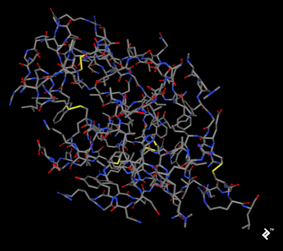
The images below, generated using the rcsb.org NGL viewer, depict the structure of experiment 132L, specifically showcasing a protein devoid of ligands. The first image utilizes a stick representation with CPK coloring, highlighting sulfurs and their bonds in yellow. V-shaped sulfur connections symbolize methionine connections, while Z-shaped connections denote disulfide bonds between cysteines.

The subsequent image employs a simplified protein visualization technique called backbone visualization, colored by amino acids, with cysteines depicted in yellow. It portrays the same protein with excluded sidechains and only a portion of its peptide group included—in this instance, the protein backbone. Composed of three atoms: N-terminal, C-alpha, and C-terminal, this representation, while lacking disulfide bonds, provides a simplified view of the protein’s spatial arrangement:

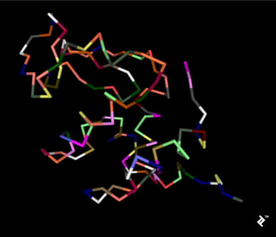
Pipes are generated by connecting peptide-bonded atoms with a C-alpha atom. The color assigned to cysteine matches that of sulfur in the CPK coloring scheme. When cysteines are in close proximity, their sulfurs form disulfide bonds, enhancing the structure’s stability. Without these bonds, the protein might exhibit excessive binding, leading to reduced stability at elevated temperatures.

CONECT

CONECT records denote connections between atoms. While these tags might be entirely absent in some cases, they can be present with complete data in others. Although potentially beneficial for disulfide bond analysis, they are not essential for this project, as non-tagged bonds are added by calculating distances. Including them would introduce unnecessary overhead and require verification.

SOURCE

These records provide information about the organism from which the molecule was extracted, incorporating subrecords for easier taxonomic classification. Similar to title records, they can span multiple lines.

 1
 2
 3
 4
 5
 6
 7
 8
 9
10

SOURCE    MOL_ID: 1;                                  
SOURCE   2 ORGANISM_SCIENTIFIC: ANOPHELES GAMBIAE;    
SOURCE   3 ORGANISM_COMMON: AFRICAN MALARIA MOSQUITO; 
SOURCE   4 ORGANISM_TAXID: 7165;                      
SOURCE   5 GENE: GST1-6;                              
SOURCE   6 EXPRESSION_SYSTEM: ESCHERICHIA COLI;       
SOURCE   7 EXPRESSION_SYSTEM_TAXID: 562;              
SOURCE   8 EXPRESSION_SYSTEM_STRAIN: BL21(DE3)PLYSS;  
SOURCE   9 EXPRESSION_SYSTEM_VECTOR_TYPE: PLASMID;    
SOURCE  10 EXPRESSION_SYSTEM_PLASMID: PXAGGST1-6      

NR Format

This section delves into the non-redundant (NR) chain PDB sets, with snapshots accessible at ftp.ncbi.nih.gov/mmdb/nrtable/. These sets aim to mitigate biases arising from protein similarity. NR comprises three sets with varying identity p-value levels generated by comparing all PDB structures. The results are compiled into textual files, which will be elaborated on subsequently. As not all columns are relevant to this project, only the essential ones will be discussed.

The first two columns contain the unique PDB experiment code and the chain identifier, as explained for ATOM records. Columns 6, 9, and C hold information regarding p-value representativeness, indicating the level of sequence similarity calculated using BLAST. A value of zero signifies exclusion from a set, while a value of one indicates inclusion. These columns represent acceptance for sets with p-value cutoffs of 10e-7, 10e-40, and 10e-80, respectively. Only sets with a p-value cutoff of 10e-7 will be employed for analysis.

The final column indicates a structure’s acceptability, where a signifies acceptable and n represents unacceptable.

1
2
3
4
5
6
7

#---------------------------------------------------------------------------------------------------------------------------
# 1  2       3     4    5 6     7    8 9     A    B C     D    E F    G      H      I      J     K     L   M   N     O P Q
#---------------------------------------------------------------------------------------------------------------------------
3F8V A   69715     1    1 1     1    1 1     1    1 1  9427    1 1   0.00   0.00   0.00   0.00  1.08   1   6   5   164 X a
3DKE X   68132     1    2 0     1    2 0     1    2 0 39139    1 1   0.00   0.00   0.00   0.00  1.25   1  11   7   164 X a
3HH3 A   77317     1    3 0     1    3 0     1    3 0    90    1 0   0.00   0.00   0.00   0.00  1.25   1   5   4   164 X a
3HH5 A   77319     1    4 0     1    4 0     1    4 0    90    2 0   0.00   0.00   0.00   0.00  1.25   1   4   4   164 X a

Database Construction and Parsing Data

Having established a basic understanding of the data and objectives, let’s proceed with the practical aspects.

Downloading Data

All data required for this analysis can be found at the following three locations:

• ftp.wwpdb.org/pub/pdb/data/structures/divided/pdb/
• ftp.ncbi.nih.gov/mmdb/nrtable/
• ftp.ncbi.nih.gov/pub/taxonomy/taxdmp.zip

The first two links provide a list of archives. Using the most recent archive from each source is recommended to avoid issues stemming from insufficient resolution or quality. The third link directly provides the newest taxonomy archive.

Parsing Data

Parsing PDB files is typically accomplished using plugins or modules in languages like Java, Perl, or Python. In this study, I developed a custom Perl application without relying on pre-built PDB-parsing modules. This decision stems from my experience with parsing large datasets, where the most prevalent issue encountered with experimental data involves data errors. These errors can manifest as coordinate discrepancies, distance inconsistencies, incorrect line lengths, misplaced comments, and more.

The most effective approach to handling such situations is to initially store all data in the database as raw text. Common parsers are designed to handle ideal, specification-compliant data. However, in practice, data often deviates from the ideal, as will be illustrated in the filtering section, where the Perl import script is presented.

Database Construction

When constructing the database, it’s crucial to recognize that its primary purpose is data processing, with subsequent analysis conducted in SPSS or R. For our needs, PostgreSQL version 8.4 or higher is recommended.

The table structure closely mirrors that of the downloaded files, with minimal modifications. In this instance, the relatively small number of records makes normalization efforts unnecessary. As mentioned earlier, this database is intended for single-use purposes, meaning the tables are not built to be served on a website. They serve as temporary structures for data processing. Once processing is complete, they can be discarded or retained as supplementary data, potentially for replication by other researchers.

In this specific scenario, the final output will be a single table, readily exportable to a file for analysis using statistical tools like SPSS or R.

Tables

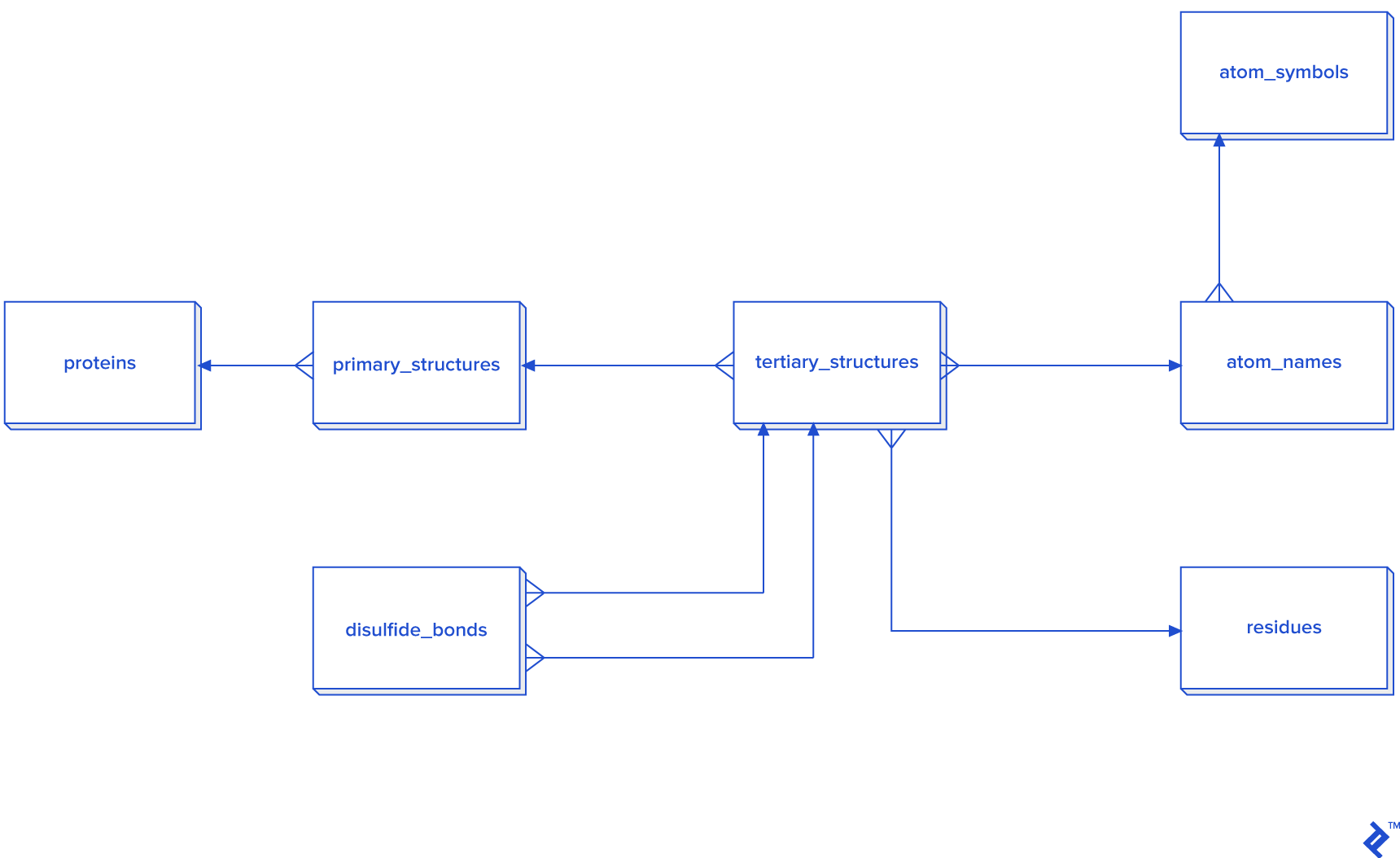
Data extracted from ATOM records must be linked to HEADER or TITLE records. The hierarchical relationship between data elements is illustrated in the diagram below.

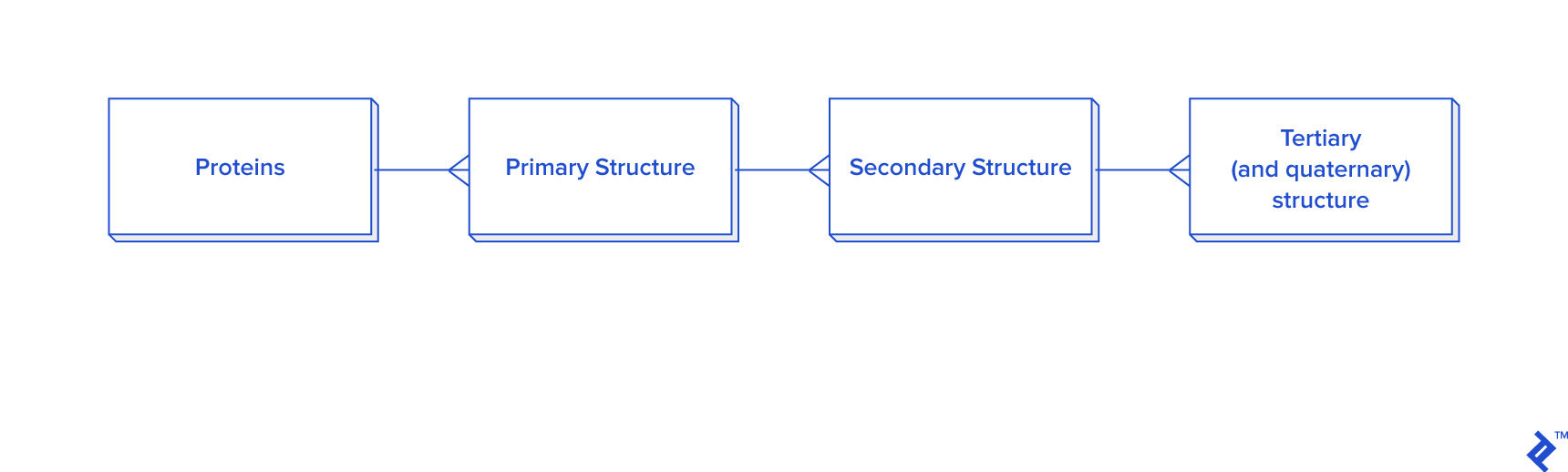
This diagram provides a simplified representation of a database in the third normal form (3NF), which introduces unnecessary overhead for our purposes. Calculating distances between atoms for disulfide bond detection would necessitate joins. In this case, we would have a table joined to itself twice, along with joins to secondary and primary structure tables, resulting in a time-consuming process. Given that secondary structure information is not always required for analysis, an alternative schema is proposed, particularly when data reuse or analysis of larger disulfide bond datasets is anticipated:

While a warehouse model is not essential for disulfide bonds, which are less frequent than other covalent bonds, it could be employed. However, developing a star schema and dimensional modeling would be overly time-consuming and introduce complexities into queries:

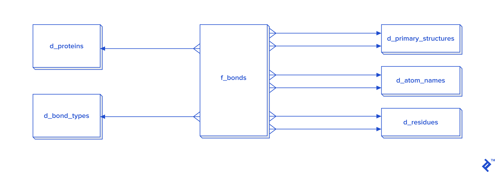
When processing all bonds is mandatory, I recommend adopting the star schema.

(Otherwise, it’s unnecessary since disulfide bonds are less prevalent compared to other bonds. In this study, with approximately 30,000 disulfide bonds, processing in 3NF might suffice, but I opted for a non-normalized table approach, hence its exclusion from the diagram.)

Considering that the estimated number of all covalent bonds is at least twice the number of atoms in the tertiary structure, a 3NF approach would be highly inefficient. Consequently, denormalization using the star schema becomes necessary. In this schema, certain tables have two foreign key checks because bonds are formed between two atoms, requiring each atom to possess its own primary_structure_id, atom_name_id, and residue_id.

There are two methods for populating the d_atom_name dimension table: using data directly or utilizing the chemical component dictionary mentioned earlier. The dictionary follows a format similar to the PDB format, with RESIDUE and CONECT lines being the most relevant. The first column of RESIDUE contains a three-letter residue code, while CONECT includes the atom name and its connections, also represented by atom names. By parsing this file, we can extract all atom names and incorporate them into our database. However, it’s advisable to accommodate the possibility of the database containing unlisted atom names.

 1
 2
 3
 4
 5
 6
 7
 8
 9
10
11
12
13
14
15
16
17
18
19
20
21
22

RESIDUE   PRO     17
CONECT      N      3 CA   CD   H   
CONECT      CA     4 N    C    CB   HA  
CONECT      C      3 CA   O    OXT 
CONECT      O      1 C   
CONECT      CB     4 CA   CG   HB2  HB3 
CONECT      CG     4 CB   CD   HG2  HG3 
CONECT      CD     4 N    CG   HD2  HD3 
CONECT      OXT    2 C    HXT 
CONECT      H      1 N   
CONECT      HA     1 CA  
CONECT      HB2    1 CB  
CONECT      HB3    1 CB  
CONECT      HG2    1 CG  
CONECT      HG3    1 CG  
CONECT      HD2    1 CD  
CONECT      HD3    1 CD  
CONECT      HXT    1 OXT 
END   
HET    PRO             17
HETNAM     PRO PROLINE
FORMUL      PRO    C5 H9 N1 O2

In this project, coding speed takes precedence over execution speed and storage consumption. Therefore, I decided against normalization, as the primary goal is to generate a table with the columns outlined in the introduction.

This section will focus on explaining the most crucial tables.

The main tables include:

• proteins: Stores experiment names and codes.
• ps: Contains the primary structure table, including sequence, chain_id, and code.
• ts: Holds the tertiary/quaternary structure extracted from raw data and transformed into the ATOM record format. It serves as a staging table and can be discarded after extraction. Ligands are excluded.
• sources: Lists the organisms from which experimental data was obtained.
• tax_names, taxonomy_path, taxonomy_paths: Contains Linnean taxonomy names from the NCBI taxonomy database, used to derive taxonomy paths for organisms listed in sources.
• nr: Stores the list of NCBI non-redundant proteins extracted from the NR set.
• pdb_ssbond: Contains the list of disulfide bonds within a given PDB file.

Filtering and Processing Data

Data retrieval is performed using snapshots from the RCSB PDB repository.

Each file is imported into a single table named raw_pdb in our PostgreSQL database using a Perl script, employing transactions of 10,000 inserts per chunk.

The structure of raw_pdb is as follows:

Below is the import script:

 1
 2
 3
 4
 5
 6
 7
 8
 9
10
11
12
13
14
15
16
17
18
19
20
21
22
23
24
25
26
27
28
29
30

#!/usr/bin/perl -w

use FindBin '$Bin';
use DBI;

$dbName = 'bioinf'; 
$dbLogin = 'ezop'; 
$dbPass = 'XYZ';

$conn = DBI->connect("DBI:Pg:database=$dbName;host=localhost", "$dbLogin", "$dbPass", {'RaiseError' => 1, 'AutoCommit' => 0});

die "./pdb_lines_unos.pl <table> <file>" if not defined($ARGV[0]);

$recordCount = 0;
$table = $ARGV[0];
$fName = $ARGV[1];
open F, "zcat $fName|";
while (<F>) {
    chomp;
    $linija = $_;
    $recordCount += 1;
    $sql = "insert into $table (code, line_num, line_cont) values (?, ?, ?)";

    $conn->do($sql, undef, $fName, $recordCount, $linija);
    $conn->commit() if ($recordCount%10000 == 0);
}
close F;
$conn->commit();

1;

After importing lines, they are parsed using functions that will be defined later.

From the data in raw_pdb, we generate the ts, ps, proteins, sources, sources_organela, and ss_bond tables by parsing their corresponding records.

The ps table comprises three essential columns: chain, length, and sequence. The protein sequence is generated using C-alpha atoms for each chain and residue, ordered by residue sequence, considering only the first insertion and alternate location. The chain value is derived from the TS.chain column, while length represents the pre-calculated length of the sequence string. As this article focuses solely on single chains and intrachain connections, proteins with multiple chains are excluded from the analysis.

All disulfide bonds within SSBOND records are stored in the pdb_ssbond table, which inherits from the pdb_ssbond_extended table. The structure of pdb_ssbond is as follows:

I have also added the following indexes:

1
2
3

"pdb_ssbond_pkey" PRIMARY KEY, btree (id)
"ndxcode1" btree (code, chain_id1, res_seq1)
"ndxcode2" btree (code, chain_id2, res_seq2)

Assuming a Gaussian distribution of disulfide bond lengths prior to cutoff (without formal testing using methods like the KS-test), standard deviations were calculated for each distance between cysteines within the same protein to determine the acceptable range of bond lengths and compare them against the cutoff. The cutoff was defined as the calculated mean plus or minus three standard deviations. To encompass more potential disulfide bonds not explicitly listed in the SSBOND rows of the PDB file, the range was extended. These bonds were identified by calculating distances between ATOM records. The chosen range for ssbonds falls between 1.6175344456264 and 2.48801947642267 Å, representing the mean (2.05) plus or minus four standard deviations:

 1
 2
 3
 4
 5
 6
 7
 8
 9
10
11
12
13
14
15
16

select                     count(1) as     cnt
    ,      stddev(dist)             as std_dev  
    ,                     avg(dist) as avg_val
    ,     -stddev(dist) + avg(dist) as   left1
    ,      stddev(dist) + avg(dist) as  right1
    , -2 * stddev(dist) + avg(dist) as   left2
    ,  2 * stddev(dist) + avg(dist) as  right2
    , -3 * stddev(dist) + avg(dist) as   left3
    ,  3 * stddev(dist) + avg(dist) as  right3
    , -4 * stddev(dist) + avg(dist) as   left4
    ,  4 * stddev(dist) + avg(dist) as  right4
    ,         min(dist)
    ,         max(dist)
from pdb_ssbond_tmp
where dist > 0
    and dist < 20;

While the TS table contains coordinates for all atoms, our analysis will focus solely on cysteines with their sulfur atom labeled as " SG ". To expedite the process, a separate staging table containing only " SG " sulfur atoms is created, reducing the number of records to be searched. By selecting only sulfurs, the number of combinations is significantly reduced from 122,761,100 (for all atoms) to 194,574. Within this self-joined table, distances are calculated using the Euclidean distance formula, and the results are imported into the pdb_ssbond table, but only if the distance falls within the predefined length range calculated earlier. This speed optimization aims to minimize the time required to rerun the entire process for verification purposes, keeping it within a one-day timeframe.

The following algorithm is employed to clean disulfide bonds:

• Delete bonds where both connection points refer to the same amino acid.
• Delete bonds with lengths outside the range of 1.6175344456264 and 2.48801947642267 Å.
• Remove insertions.
• Remove bonds resulting from alternate atom locations, retaining only the first location.

The code implementing this algorithm (taking the pdb_ssbond table as the first argument) is as follows:

  1
  2
  3
  4
  5
  6
  7
  8
  9
 10
 11
 12
 13
 14
 15
 16
 17
 18
 19
 20
 21
 22
 23
 24
 25
 26
 27
 28
 29
 30
 31
 32
 33
 34
 35
 36
 37
 38
 39
 40
 41
 42
 43
 44
 45
 46
 47
 48
 49
 50
 51
 52
 53
 54
 55
 56
 57
 58
 59
 60
 61
 62
 63
 64
 65
 66
 67
 68
 69
 70
 71
 72
 73
 74
 75
 76
 77
 78
 79
 80
 81
 82
 83
 84
 85
 86
 87
 88
 89
 90
 91
 92
 93
 94
 95
 96
 97
 98
 99
100
101
102
103
104
105
106
107
108
109
110
111
112
113
114
115
116
117
118
119
120
121
122
123
124
125
126
127
128
129
130
131
132
133
134
135
136
137
138
139
140
141
142
143
144
145
146
147
148
149
150
151
152
153
154
155
156

 CREATE OR REPLACE FUNCTION pdb_ssbond_clean2( 
    clean_icodes boolean,
    clean_altloc boolean,
    mark_reactive boolean,
    mark_consecutive boolean)
RETURNS void AS $
declare _res integer;
BEGIN  
    delete from pdb_ssbond b 
    where exists (
        select a.id
        from pdb_ssbond a
        where a.code = b.code
        and a.id > b.id
        and (
            (   a.chain_id1 = b.chain_id1 and a.res_seq1 = b.res_seq1
            and a.chain_id2 = b.chain_id2 and a.res_seq2 = b.res_seq2)
            or
            (   a.chain_id1 = b.chain_id2 and a.res_seq1 = b.res_seq2
            and a.chain_id2 = b.chain_id1 and a.res_seq2 = b.res_seq1)
        )
    ) ; 

    delete
    from pdb_ssbond
    where chain_id1 = chain_id2
    and res_seq1 = res_seq2
    and i_code1 = i_code2;
        
 
         
    update pdb_ssbond 
    set is_consecutive = true
    , is_reactive = false;
        
    delete from pdb_ssbond 
    where not dist between 1.6175344456264 and 2.48801947642267;
     
          
    
    if clean_icodes then  
        delete from pdb_ssbond 
        where  i_code1 not in ('',  ' ', 'A') 
        or     i_code2 not in ('',  ' ', 'A') ;
    end if;
    
    if clean_altloc then  
        delete from pdb_ssbond a
        where exists (
            select 1
            from pdb_ssbond  b
            where   b.code = a.code
                and b.chain_id1 = a.chain_id1
                and b.res_seq1 = a.res_seq1
                and b.i_code1 = a.i_code1
                and b.ser_num < a.ser_num
        ) ;
        
        delete from pdb_ssbond a
        where exists (
            select 1
            from pdb_ssbond  b
            where   b.code = a.code
                and b.chain_id2 = a.chain_id2
                and b.res_seq2 = a.res_seq2
                and b.i_code2 = a.i_code2
                and b.ser_num < a.ser_num
        ) ;
    end if;

    if mark_reactive then  
            update pdb_ssbond 
            set is_reactive = false ; 
       
            update pdb_ssbond 
            set is_reactive = true
            where exists (
                select 1
                from pdb_ssbond  b
                where   b.code = pdb_ssbond.code
                    and b.chain_id1 = pdb_ssbond.chain_id1
                    and b.res_seq1 = pdb_ssbond.res_seq1
                    and b.i_code1 = pdb_ssbond.i_code1
                    and b.ser_num < pdb_ssbond.ser_num
            ) ;  
         
       
            update pdb_ssbond 
            set is_reactive = true         
            where exists (
                select 1
                from pdb_ssbond  b
                where   b.code = pdb_ssbond.code
                    and b.chain_id2 = pdb_ssbond.chain_id2
                    and b.res_seq2 = pdb_ssbond.res_seq2
                    and b.i_code2 = pdb_ssbond.i_code2
                    and b.ser_num < pdb_ssbond.ser_num
            ) ; 
       
            update pdb_ssbond 
            set is_reactive = true         
            where (code, chain_id1, res_seq1, i_code1)
            in (
                select code, chain_id1 as c, res_seq1 as r, i_code1 as i
                from pdb_ssbond
                intersect
                select code, chain_id2 as c, res_seq2 as r, i_code2 as i
                from pdb_ssbond
            ) ; 
       
 
            update pdb_ssbond 
            set is_reactive = true         
            where (code, chain_id2, res_seq2, i_code2)
            in (
                select code, chain_id1 as c, res_seq1 as r, i_code1 as i
                from pdb_ssbond
                intersect
                select code, chain_id2 as c, res_seq2 as r, i_code2 as i
                from pdb_ssbond
            );
    end if;
    
    if mark_consecutive then
           update pdb_ssbond
           set is_consecutive = false;

            update pdb_ssbond
            set is_consecutive = true
            where not exists (
                select 1
                from pdb_ssbond a
                where
                    a.code = pdb_ssbond.code
                    and (
                        (a.chain_id1 = pdb_ssbond.chain_id1 and a.chain_id2 = pdb_ssbond.chain_id2)
                        or
                        (a.chain_id1 = pdb_ssbond.chain_id2 and a.chain_id2 = pdb_ssbond.chain_id1)
                    )
                    and (
                           (a.res_seq1 between pdb_ssbond.res_seq1 and pdb_ssbond.res_seq2)
                        or (a.res_seq2 between pdb_ssbond.res_seq1 and pdb_ssbond.res_seq2)
                        or (pdb_ssbond.res_seq1 between a.res_seq1 and a.res_seq2)
                        or (pdb_ssbond.res_seq2 between a.res_seq1 and a.res_seq2)
                    )
                    and not (
                            a.code = pdb_ssbond.code
                        and a.chain_id1 = pdb_ssbond.chain_id1
                        and a.chain_id2 = pdb_ssbond.chain_id2 
                        and a.res_seq1 = pdb_ssbond.res_seq1
                        and a.res_seq2 = pdb_ssbond.res_seq2
                    )
            );
    end if; 
END;
$ LANGUAGE plpgsql;

Subsequently, the non-redundant set of proteins is imported into the nr table, which is then joined with the ps and proteins tables. Sets are marked using set7, set40, and set80. Ultimately, only one set will be analyzed based on protein quantity. Any mismatched chains between PDB and NR are excluded from the analysis.

Proteins lacking disulfide bonds are removed from the study, along with those not belonging to any set. Data is processed using DSSP, and proteins exhibiting resolution issues or an excessive number of atoms are also excluded. Only proteins with single chains are retained for analysis, as interchain connections are not maintained, although they can be easily calculated from the ssbond table by counting connections with different chains.

For the remaining proteins, the total number of bonds and overlapping bonds are updated for each set.

The source organism is extracted from SOURCE records. Entries marked as unknown, synthetic, designed, artificial, or hybrid are discarded from the study. Low-resolution proteins are excluded only if their side chains are not visible.

SOURCE records are stored in the sources table, which includes taxonomy rows. In cases of missing or incorrect taxonomy information, manual correction by experts is required.

Based on the source and taxonomy information downloaded from NCBI, each primary structure is assigned a class. Proteins with unassigned classes are removed from the analysis list. Due to the reliance on biological databases, it is highly recommended that a biologist performs an additional verification of all source records and NCBI taxonomy classifications to avoid potential misclassifications between different domains.

To map source cellular locations to taxonomy IDs, data from the source table is extracted into the sources_organela table, where all data is represented using codes, tags, and values. Its format is shown below:

1

select * from sources_organela where code = '1rav';

The taxonomy archive used in this study is a ZIP file containing seven dump files. Among these, names.dmp and merged.dmp are particularly important. Both are CSV files using tab and pipe delimiters as detailed in the documentation:

• merged.dmp provides a mapping of previous taxonomy IDs to their current counterparts.
• names.dmp contains the following essential columns in the specified order:
  • tax_id: The taxonomy ID.
  • name_txt: The species name and, if applicable, the unique name (used for disambiguation when multiple names exist for a species).
• division.dmp contains the names of top-level domains, which will serve as our classes.
• nodes.dmp represents the hierarchical structure of organisms based on taxonomy IDs.
  • It includes a parent taxonomy ID, serving as a foreign key referencing names.dmp.
  • It also contains a division ID, crucial for storing relevant top-domain data.

Using this data and manual corrections (to ensure accurate domains of life assignments), we constructed the taxonomy_path table. A sample of the data is shown below:

1

select * from taxonomy_path order by length(path)  limit 20 offset 2000;

To mitigate biases, sequences must undergo identity level checks before analysis. Although the NR set contains pre-compared sequences, an additional verification is always recommended.

For statistical analysis of each disulfide bond, data is tagged as reactive or overlapping. By marking overlaps, we automatically determine the number of consecutive and non-consecutive bonds within each protein. This information is stored in the proteins table, from which all protein complexes are excluded in the final results.

Each disulfide bond is also associated with sets by checking if both bond sides belong to the same NR set. Bonds with sides belonging to different sets are omitted from the analysis for that specific set.

Analyzing the quantity of bonds based on their variance requires categorizing each length into a specific class. In this study, we used five classes, as defined in the function below:

 1
 2
 3
 4
 5
 6
 7
 8
 9
10
11
12
13
14
15
16

CREATE OR REPLACE FUNCTION len2class(len integer)
    RETURNS integer AS
$BODY$
BEGIN
return 
    case 
        when len <= 100                then 1
        when len >  100 and len <= 200 then 2
        when len >  200 and len <= 300 then 3
        when len >  300 and len <= 400 then 4
                                       else 5
    end;
END;
$BODY$
    LANGUAGE plpgsql VOLATILE
    COST 100;

Since most protein sizes are below 400 amino acids, length classification is performed by dividing lengths into five ranges. The first four ranges span 100 amino acids each, while the last range encompasses the remaining lengths. The following code snippet demonstrates how to utilize this function for data extraction and analysis:

 1
 2
 3
 4
 5
 6
 7
 8
 9
10
11
12
13
14
15
16
17
18
19
20
21
22
23
24
25
26
27
28
29
30
31

 SELECT p.code,
    p.title,
    p.ss_bonds,
    p.ssbonds_overlap,
    p.intra_count,
    p.sci_name_src,
    p.len,
    p.tax_path,
    p.pfam_families,
    p.src_class,
    ( SELECT s.id
           FROM src_classes s
          WHERE s.src_class::text = p.src_class::text) AS src_class_id,
    p.len_class7,
    ( SELECT s.val
           FROM sources_organela s
          WHERE s.code = p.code::bpchar AND s.tag::text = 'EXPRESSION_SYSTEM_CELLULAR_LOCATION'::text) AS expression_system_cellular_location,
    ( SELECT s.val
           FROM sources_organela s
          WHERE s.code = p.code::bpchar AND s.tag::text = 'CELLULAR_LOCATION'::text) AS cellular_location,
    ps.sequence,
    ps.uniprot_code,
    ps.accession_code,
    ps.cc,
    ps.seq_uniprot,
    ps.chain_id
   FROM proteins p
     JOIN nr n ON n.code::text = p.code::text AND n.rep7 = true
     JOIN ps ps ON ps.code::text = n.code::text AND ps.chain_id = n.chain_id AND ps.het = false
  WHERE p.is_excluded = false AND p.chain_cnt = 1 AND p.is_set7 = true AND p.reactive_cnt7 = 0
  ORDER BY p.code;

An example of the output, incorporating corrected titles and manually added columns, is provided below:

PostgreSQL as a Processing Intermediary

This work outlined a comprehensive data processing pipeline, from fetching to analysis. In scientific data analysis, normalization might not always be necessary. When dealing with small datasets intended for one-time analysis, denormalization can be sufficient if processing speed is adequate.

The decision to perform all processing within a single bioinformatics database stems from PostgreSQL’s ability to integrate with various languages, including R. This enables statistical analysis directly within the database—a topic for a future article on bioinformatics tools.

Special thanks to my Toptal colleagues Stefan Fuchs and Aldo Zelen for their invaluable insights and consultations.