Currently, being a Data Scientist is quite advantageous. Discussing “Big Data” piques the interest of serious individuals, while mentioning “Artificial Intelligence” and “Machine Learning” captivates the attention of partygoers. Even Google thinks you’re improving constantly. Numerous ‘smart’ algorithms assist data scientists in their craft. Although seemingly complex, understanding and categorizing these algorithms simplifies the process of finding and applying the appropriate one.

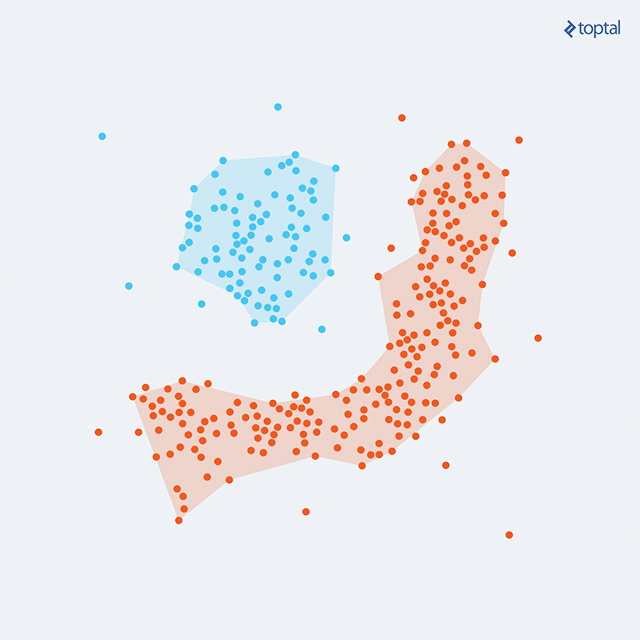
Data mining or machine learning courses typically begin with clustering due to its simplicity and practicality. As a crucial element of Unsupervised Learning, it deals with unlabeled data. This often implies that limited information is provided regarding the anticipated output. The algorithm, solely relying on the data, must strive for optimal results. In clustering, this involves segregating data into clusters containing similar data points while maximizing dissimilarity between groups. These data points can symbolize anything, even customers. For instance, clustering helps group similar users, enabling targeted marketing campaigns for each cluster.

K-Means Clustering

Data Mining courses consistently introduce K-Means after the initial concepts. This algorithm, renowned for its effectiveness and widespread use, proves highly versatile in clustering. Prior to execution, defining a distance function between data points (e.g., Euclidean distance for clustering points in space) and setting the desired number of clusters (k) are essential.

The algorithm starts by choosing k points as initial centroids, representing cluster ‘centers’. Randomly selecting any k points is a viable option, although other approaches exist. Subsequently, two steps are repeated iteratively:

1. Assignment step: Each of the m data points is assigned to the cluster whose centroid is nearest. Distances between each point and every centroid are calculated, with the least distant centroid determining the cluster assignment.

2. Update step: For each cluster, a new centroid is computed as the average of all points within that cluster. Using the point assignments from the previous step, a mean is calculated for each set of points, establishing the new cluster centroid.

With each iteration, centroids gradually shift, reducing the total distance between points and their assigned centroids. These steps alternate until convergence until cluster assignments stabilize. After several iterations, identical point sets will be allocated to each centroid, resulting in static centroids. K-Means guarantees convergence to a local optimum, but not necessarily the best overall solution (global optimum).

As the final clustering outcome can be influenced by the initial centroid selection, significant attention has been dedicated to this aspect. Running K-Means multiple times with random initial assignments presents a simple solution. Choosing the result with the smallest total distance between points and their clusters—the error value being minimized—yields the optimal outcome.

Other approaches leverage distant point selection for initial points. While potentially improving results, outliers—rare, isolated points potentially representing errors—can pose challenges. Being distant from significant clusters, these points might form individual ‘clusters’. The K-Means++ variant [Arthur and Vassilvitskii, 2007] offers a good balance. While still randomly selecting initial points, the probability is proportional to the squared distance from previously assigned centroids. Consequently, distant points have a higher probability of becoming initial centroids. Furthermore, the probability of selecting a point within a group increases as their probabilities combine, addressing the outlier issue.

K-Means++ also serves as the default initialization for Python’s Scikit-learn K-Means implementation, a potentially preferred library for Python users. For Java, the Weka library is a suitable starting point:

Java (Weka)

 1
 2
 3
 4
 5
 6
 7
 8
 9
10
11
12
13
14
15
16
17
18
19
20
21
22

// Load some data
Instances data = DataSource.read("data.arff");

// Create the model
SimpleKMeans kMeans = new SimpleKMeans();

// We want three clusters
kMeans.setNumClusters(3);

// Run K-Means
kMeans.buildClusterer(data);

// Print the centroids
Instances centroids = kMeans.getClusterCentroids();
for (Instance centroid: centroids) {
  System.out.println(centroid);
}

// Print cluster membership for each instance
for (Instance point: data) {
  System.out.println(point + " is in cluster " + kMeans.clusterInstance(point));
}

Python (Scikit-learn)

 1
 2
 3
 4
 5
 6
 7
 8
 9
10
11
12

> >> from sklearn import cluster, datasets
> >> iris = datasets.loadiris()
> >> Xiris = iris.data
> >> yiris = iris.target

> >> kmeans = cluster.KMeans(nclusters=3)
> >> kmeans.fit(Xiris)
KMeans(copy_x=True, init='k-means++', ...
> >> print(kmeans.labels[::10])
[1 1 1 1 1 0 0 0 0 0 2 2 2 2 2]
> >> print(yiris[::10])
[0 0 0 0 0 1 1 1 1 1 2 2 2 2 2]

The Python example demonstrates the use of the ‘Iris’ dataset, containing flower petal and sepal dimensions for three iris species. Clustering these into three clusters and comparing them to the actual species (target) reveals a perfect match.

In this scenario, the existence of three distinct clusters (species) was known, and K-Means accurately identified them. However, determining an appropriate cluster number (k) generally poses a common challenge in Machine Learning. Increasing the cluster count reduces cluster size, thereby minimizing the total error (total distance of points to their clusters). This raises the question: Is simply increasing k a viable solution? Setting k equal to m results in each point becoming its own centroid, with each cluster containing a single point. While the total error is zero, this approach fails to provide a simpler data representation or generalize to new data points, leading to overfitting—an undesirable outcome.

Addressing this issue involves incorporating a penalty for a larger number of clusters. Consequently, the minimization target becomes error + penalty. While increasing the cluster count drives the error towards zero, the penalty increases. At a certain point, the gain from adding another cluster is outweighed by the penalty, yielding the optimal result. X-Means [Pelleg and Moore, 2000], utilizing the Bayesian Information Criterion (BIC) for this purpose, embodies such a solution.

Properly defining the distance function is crucial. While straightforward in some cases (e.g., Euclidean distance for spatial points), it can be complex for features with different ‘units’, discrete variables, etc., demanding significant domain expertise. Alternatively, Machine Learning can assist in learning the distance function. Utilizing a training set of points with known groupings (labeled with their clusters), supervised learning techniques can identify a suitable function, which can then be applied to the unclustered target set.

The two-step alternating method employed in K-Means resembles the Expectation–Maximization (EM) method, essentially a simplified EM version. However, it should not be confused with the more sophisticated EM clustering algorithm despite sharing some principles.

EM Clustering

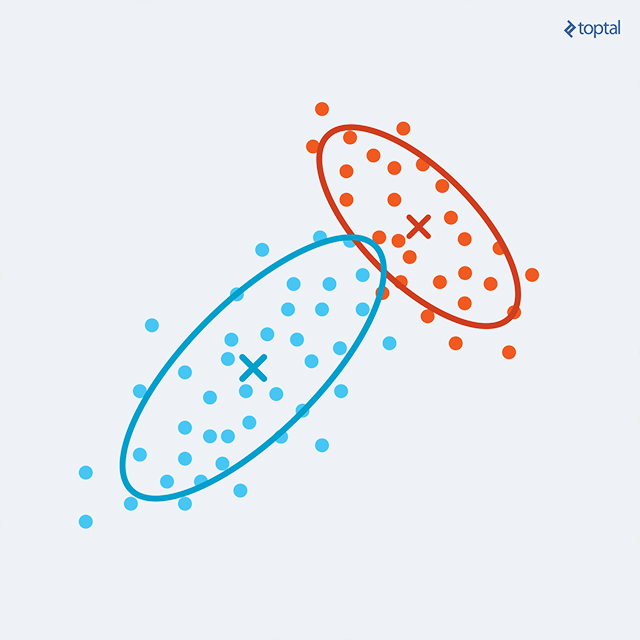
In K-Means clustering, each point is assigned to a single cluster, with the centroid solely describing the cluster. This approach lacks flexibility, potentially causing issues with overlapping or non-circular clusters. EM Clustering enhances this by representing each cluster with its centroid (mean), covariance (allowing elliptical clusters), and weight (cluster size). The probability of a point belonging to a cluster is now determined by a multivariate Gaussian probability distribution (multivariate due to dependence on multiple variables). This enables the calculation of the probability of a point falling under a Gaussian ‘bell’, representing the probability of cluster membership.

The EM procedure begins by calculating the probabilities of each point belonging to each existing cluster (potentially randomly generated initially). This constitutes the E-step. A high probability (close to one) indicates a strong cluster candidacy for a point. However, as multiple clusters might be suitable candidates, the point possesses a probability distribution across clusters. This characteristic, where points are not restricted to a single cluster, is termed “soft clustering”.

In the M-step, each cluster’s parameters are recalculated based on point assignments from the preceding clusters. Point data is weighted by its probability of belonging to the cluster (calculated in the E-step) when computing the new mean, covariance, and weight.

Alternating these steps increases the total log-likelihood until convergence. As the maximum can be local, running the algorithm multiple times might yield superior clusters.

To determine a single cluster for each point, the most probable cluster can be selected. The probability model also facilitates the generation of similar data by sampling more points resembling the observed data.

Affinity Propagation

Published in 2007 by Frey and Dueck, Affinity Propagation (AP) is gaining popularity due to its simplicity, general applicability, and performance. It is transitioning from a cutting-edge technique to a standard approach.

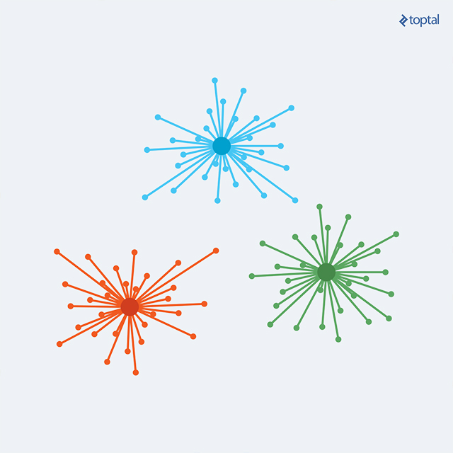
K-Means and similar algorithms suffer from the need to predefine the number of clusters and select initial points. Conversely, Affinity Propagation utilizes pairwise data point similarity measures as input and simultaneously considers all points as potential exemplars. Real-valued messages are exchanged between data points, progressively revealing a high-quality set of exemplars and their corresponding clusters.

The algorithm requires two input datasets:

1. Similarities between data points: Representing the suitability of a point as another point’s exemplar. Lack of similarity, indicating points cannot belong to the same cluster, can be represented by omission or -Infinity, depending on the implementation.

2. Preferences: Reflecting each point’s suitability to be an exemplar. Existing a priori information favoring certain points for this role can be incorporated through preferences.

A single matrix often represents both similarities and preferences, with diagonal values representing preferences. This matrix representation suits dense datasets. For sparse point connections, storing a list of similarities to connected points proves more practical than storing the entire n x n matrix. “Exchanging messages between points” conceptually mirrors matrix manipulation, differing only in perspective and implementation.

The algorithm iterates until convergence, with each iteration involving two message-passing steps:

1. Calculating responsibilities: Responsibility r(i, k) quantifies the cumulative evidence supporting point k’s suitability as the exemplar for point i, considering other potential exemplars for point i. Responsibility is transmitted from data point i to candidate exemplar point k.

2. Calculating availabilities: Availability a(i, k) quantifies the cumulative evidence supporting point i choosing point k as its exemplar, considering the support from other points for point k’s exemplar candidacy. Availability is transmitted from candidate exemplar point k to point i.

Responsibility calculation utilizes original similarities and availabilities from the previous iteration (initially, all availabilities are zero). Responsibility is assigned the input similarity between point i and point k as its exemplar, minus the largest value among the similarity and availability sum between point i and other candidate exemplars. This calculation logic favors higher initial a priori preferences. However, the presence of a similar point considering itself a strong candidate lowers the responsibility, resulting in ‘competition’ until one point is favored in a certain iteration.

Availability calculation leverages calculated responsibilities as evidence for each candidate’s exemplar suitability. Availability a(i, k) is set as the self-responsibility r(k, k) plus the sum of positive responsibilities received by candidate exemplar k from other points.

Finally, various stopping criteria, such as value changes falling below a threshold or reaching the maximum iteration count, can terminate the procedure. Throughout Affinity Propagation, summing Responsibility (r) and Availability (a) matrices provides the necessary clustering information: for point i, the k with the maximum r(i, k) + a(i, k) represents point i’s exemplar. Alternatively, scanning the main diagonal identifies the exemplar set; if r(i, i) + a(i, i) > 0, point i is an exemplar.

While K-Means and similar algorithms present challenges in determining the optimal cluster count, AP eliminates this explicit specification. However, tuning might be necessary if the resulting cluster count deviates from the desired outcome. Fortunately, adjusting preferences can manipulate the cluster count. Higher preferences lead to more clusters, as each point becomes ‘more certain’ of its exemplar suitability, making it harder to ‘beat’ and include under another point’s ‘domination’. Conversely, lower preferences result in fewer clusters, as if points are relinquishing their exemplar candidacy in favor of another. As a general guideline, setting preferences to the median similarity yields a medium to large cluster count, while the lowest similarity results in a moderate count. Nevertheless, several runs with preference adjustments might be needed to achieve the desired outcome.

Hierarchical Affinity Propagation, a notable variant, addresses quadratic complexity by partitioning the dataset into subsets, clustering them individually, and performing a second-level clustering.

In The End…

Numerous clustering algorithms exist, each with its strengths and weaknesses regarding suitable data types, time complexity, and limitations. For instance, Hierarchical Agglomerative Clustering (or Linkage Clustering) excels when dealing with non-circular (or non-hyperspherical) clusters and an unknown cluster count. Starting with each point as a separate cluster, it merges the two closest clusters iteratively until all points belong to a single cluster.

Hierarchical Agglomerative Clustering allows easy determination of the cluster count by horizontally cutting the dendrogram (tree diagram) at a suitable level. While ensuring repeatability (consistent results for the same dataset), it exhibits higher complexity (quadratic).

DBSCAN (Density-Based Spatial Clustering of Applications with Noise) is another noteworthy algorithm. Grouping densely packed points and expanding clusters in directions with nearby points, it handles diverse cluster shapes effectively.

These algorithms warrant dedicated articles for comprehensive exploration.

Knowing when to utilize a specific algorithm often requires experience and experimentation. Fortunately, diverse implementations across various programming languages exist, requiring only a willingness to explore and experiment.