It’s widely acknowledged that microservices application architecture is becoming increasingly prevalent in software design. This approach offers numerous advantages, including efficient load distribution, high-availability deployments, simplified upgrades, and streamlined development and team management.

However, this architectural style wouldn’t be nearly as powerful without container orchestrators.

The allure of leveraging all the features of container orchestrators, particularly auto-scaling, is undeniable. Witnessing container deployments dynamically adjust throughout the day, seamlessly scaling to accommodate current load demands, is truly remarkable. This automated process frees up valuable time for other tasks. We find ourselves incredibly satisfied with the insights provided by our container monitoring tools, knowing that we’ve achieved this level of efficiency with just a few configuration settings—it’s almost like magic!

This sense of accomplishment is well-deserved. We can confidently assert that our users are enjoying a seamless experience without incurring unnecessary expenses from oversized infrastructure. This alone is a significant achievement.

However, the journey to reach this point is not without its challenges. While the final configuration may appear deceptively simple, the process of getting there is far more intricate than one might initially anticipate. Parameters such as the minimum and maximum number of replicas, upscale and downscale thresholds, synchronization periods, and cooldown delays are intricately interconnected. Adjusting one parameter often has cascading effects on others, necessitating a delicate balancing act to find the optimal combination that aligns with both your application’s deployment requirements and your infrastructure’s capabilities. Unfortunately, there is no one-size-fits-all solution or magical formula available online, as the ideal configuration hinges largely on your unique needs.

In most cases, we start with arbitrary or default values and fine-tune them based on observations gathered through monitoring. This trial-and-error approach led me to ponder: Could we devise a more systematic, mathematically-grounded procedure to help us determine the optimal parameter combination?

Determining Container Orchestration Parameters

When considering auto-scaling for microservices within an application, our primary objectives are twofold:

1. Ensuring rapid deployment scale-up capabilities to handle sudden surges in load, preventing user timeouts or HTTP 500 errors.
2. Minimizing infrastructure costs by preventing instances from being underutilized.

Essentially, this translates to optimizing the thresholds that trigger the scaling up and down of container software. (Note: Kubernetes’ algorithm utilizes a single parameter for both scaling directions).

I will elaborate later on how all instance-specific parameters are inherently linked to the upscale threshold. This particular threshold presents the most significant challenge in calculation, hence the focus of this article.

Important: For parameters applied cluster-wide, I haven’t established a concrete procedure. However, at the conclusion of this article, I will introduce a software tool (a static web page) that incorporates these parameters while calculating an instance’s auto-scaling settings. This tool will allow you to experiment with different values and observe their impact.

Determining the Scale-up Threshold

To effectively utilize this method, your application must fulfill the following prerequisites:

1. Uniform load distribution across all instances of your application (typically achieved through a round-robin mechanism).
2. Request processing times shorter than your container cluster’s load-check interval.
3. Consideration of a substantial number of users when running this procedure (more on this later).

These conditions stem from the fact that the algorithm calculates load distribution rather than load per user, as explained further below.

Embracing the Gaussian Distribution

Our first step involves defining a “rapid load increase,” essentially a worst-case scenario. A suitable interpretation could be: a large number of users simultaneously initiating resource-intensive actions, potentially coinciding with other user groups or services performing their own tasks. Let’s translate this definition into mathematical terms (brace yourself!).

Let’s introduce some variables:

• $N_{u}$ represents the “large number of users.”
• $L_{u}(t)$ represents the load generated by a single user executing the “resource-consuming operation” (with $t=0$ indicating the operation’s start time).
• $L_{tot}(t)$ denotes the total load generated by all users.
• $T_{tot}$ signifies the “short period of time.”

In the realm of mathematics, when a large number of users engage in the same activity simultaneously, their distribution over time often resembles a Gaussian (or normal) distribution, mathematically represented as:

[G(t) = \frac{1}{\sigma \sqrt{2 \pi}} e^{\frac{-(t-\mu)^2}{2 \sigma^2}}]

Where:

• µ denotes the expected value.
• σ represents the standard deviation.

The graphical representation of this function (with $µ=0$) is as follows:

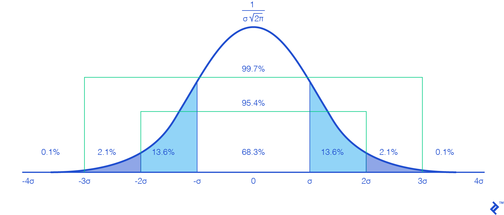
This might seem familiar from your math classes – nothing groundbreaking here. However, we encounter our first hurdle: For mathematical accuracy, we should ideally consider a time range spanning from $-\infty$ to $+\infty$, which is computationally impossible.

Examining the graph, we observe that values outside the interval $[-3σ, 3σ]$ approach zero and exhibit minimal variation, implying a negligible impact that can be safely disregarded. This simplification is further justified by our objective of testing the scale-up capacity, focusing on scenarios with substantial user fluctuations.

Furthermore, considering that the interval $[-3σ, 3σ]$ encompasses 99.7 percent of our user base, it provides a sufficiently accurate representation of the total. To compensate for the minor discrepancy, we can multiply $N_{u}$ by 1.003. By selecting this interval, we establish $µ=3σ$ (as our calculations begin at $t=0$).

Regarding the relationship with $T_{tot}$, setting it equal to $6σ$ ($[-3σ, 3σ]$) wouldn’t be entirely accurate. Approximately 95.4 percent of users fall within the interval $[-2σ, 2σ]$, spanning $4σ$. Therefore, choosing $T_{tot}$ as $6σ$ would add half the time for a mere 4.3 percent of users, lacking representativeness. Consequently, we opt for $T_{tot}=4σ$, leading to the following deductions:

\(σ=\frac{T_{tot}}{4}\) and \(µ=\frac{3}{4} * T_{tot}\)

Were these values arbitrarily chosen? Indeed. However, that is precisely their purpose, and it won’t affect the mathematical procedure itself. These constants serve as our definitions, shaping the parameters of our hypothesis. With them established, our worst-case scenario can be articulated as:

The load produced by 99.7 percent of $N{u}$, all executing the resource-intensive operation $L{u}(t)$, with 95.4 percent completing it within the timeframe $T{tot}$.

(It’s crucial to bear this in mind when utilizing the web application later on.)

Plugging these results back into the Gaussian user distribution function, we can simplify the equation:

[G(t) = \frac{4 N_{u}}{T_{tot} \sqrt{2 \pi}} e^\frac{-(4t-3T_{tot})^2}{T_{tot}^2}]

With $σ$ and $µ$ defined, our focus will be on the interval $t \in [0, \frac{3}{2}T_{tot}]$ (covering $6σ$).

Determining Total User Load

The next step in fine-tuning microservices auto-scaling involves calculating $L_{tot}(t)$.

Given that $G(t)$ represents a distribution, determining the number of users at a specific time point necessitates calculating its integral (or utilizing its cumulative distribution function). However, directly incorporating $L_{u}(t)$ and simplifying the equation to a usable formula would prove exceedingly complex due to the staggered start times of user operations.

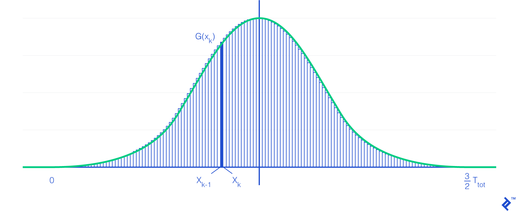
To simplify this process, we’ll employ a Riemann sum. This mathematical technique approximates an integral using a finite sum of simple shapes (in our case, rectangles). A higher number of subdivisions (shapes) results in greater accuracy. An additional advantage of subdivisions is that we can assume all users within a given subdivision initiate their operations concurrently.

Returning to the Riemann sum, it exhibits the following relationship with integrals:

[\int_{a}^{b} f( x )dx = \lim_{n \rightarrow \infty } \sum_{k=1}^{n} ( x_{k} - x_{k-1} )f( x_{k} )]

With $x_k$ defined as:

[x_{ k } = a + k\frac{ b - a }{ n }, 0 \leq k \leq n]

This holds true where:

• $n$ is the number of subdivisions.
• $a$ represents the lower bound, in this case, 0.
• $b$ represents the upper bound, here $\frac{3}{2}*T_{tot}$.
• $f$ is the function (in our case, $G$) whose area we aim to approximate.

Important Note: The number of users within a subdivision may not be a whole number. This highlights the importance of two prerequisites: a sufficiently large number of users (minimizing the impact of decimals) and uniform load distribution across instances.

Observe how the right-hand side of the Riemann sum definition visually represents the rectangular shape of each subdivision.

Armed with the Riemann sum formula, we can express the load at time $t$ as the sum of the number of users in each subdivision multiplied by the user load function at their respective times. Mathematically:

[L_{ tot }( t ) = \lim_{n \rightarrow \infty} \sum_{ k=1 }^{ n } ( x_{k} - x_{k-1} )G( x_{k} )L_{ u }( t - x_{k} )]

Substituting variables and simplifying the formula yields:

[L_{ tot }( t ) = \frac{6 N_{u}}{\sqrt{2 \pi}} \lim_{n \rightarrow \infty} \sum_{ k=1 }^{ n } (\frac{1}{n}) e^{-{(\frac{6k}{n} - 3)^{2}}} L_{ u }( t - k \frac{3 T_{tot}}{2n} )]

There you have it—our load function!

Pinpointing the Scale-up Threshold

The final step involves running a dichotomy algorithm, which systematically adjusts the threshold to identify the highest value that prevents the load per instance from exceeding its maximum limit throughout the entire load function. (The web application we’ll introduce handles this calculation).

Deriving Other Orchestration Parameters

Once you’ve determined your scale-up threshold ($S_{up}$), calculating the remaining parameters becomes relatively straightforward.

The $S_{up}$ value will reveal your maximum number of instances. (Alternatively, you can find the peak load on your load function and divide it by the maximum load permissible per instance, rounding up the result).

The minimum number of instances ($N_{min}$) should be determined based on your infrastructure. (A common recommendation is at least one replica per Availability Zone). However, it’s also crucial to factor in the load function’s characteristics. Since a Gaussian function rises quite steeply, the initial load distribution per replica is more concentrated. Therefore, consider increasing the minimum number of replicas to mitigate this effect. (This adjustment will likely impact your $S_{up}$ value).

Lastly, after defining the minimum number of replicas, you can calculate the scale-down threshold ($S_{down}$) with this consideration: The impact of scaling down a single replica on other instances is comparable to scaling down from $N_{min}+1$ to $N_{min}$. Therefore, we must ensure that the scale-up threshold doesn’t trigger immediately after a scale-down, preventing a yo-yo effect. In essence:

[( N_{ min } + 1) S_{ down } < N_{ min }S_{ up }]

Or, equivalently:

[S_{ down } < \frac{N_{ min }}{N_{min}+1}S_{ up }]

Logically, a longer waiting period before scaling down, as configured in your cluster, allows for setting $S_{down}$ closer to its upper limit. Again, finding the right balance for your specific needs is key.

Note that when utilizing the Mesosphere Marathon orchestration system with its autoscaler, the maximum number of instances removable at once during scaling down is governed by AS_AUTOSCALE_MULTIPLIER ($A_{mult}$), leading to:

[S_{ down } < \frac{S_{ up }}{ A_{mult} }]

Addressing the User Load Function

Indeed, this aspect presents a significant challenge, and it’s not easily solvable through purely mathematical means—if at all.

As a workaround, one approach involves running a single instance of your application and progressively increasing the number of users performing the same task repeatedly. Continue this until the server load reaches its assigned maximum without exceeding it. Then, divide by the number of users and compute the average request processing time. Repeat this process for each action you intend to incorporate into your user load function, incorporate timing considerations, and you’re set.

While this method operates under the assumption of constant load per user request throughout its processing (which isn’t entirely accurate), the sheer volume of users should average out this effect, as they won’t all be at the same processing stage simultaneously. Therefore, this approximation can be deemed acceptable, but it underscores the importance of dealing with a substantial user base.

Feel free to explore alternative methods, like CPU flame graphs. However, establishing a precise formula that directly correlates user actions to resource consumption will likely prove quite difficult.

Introducing the app-autoscaling-calculator

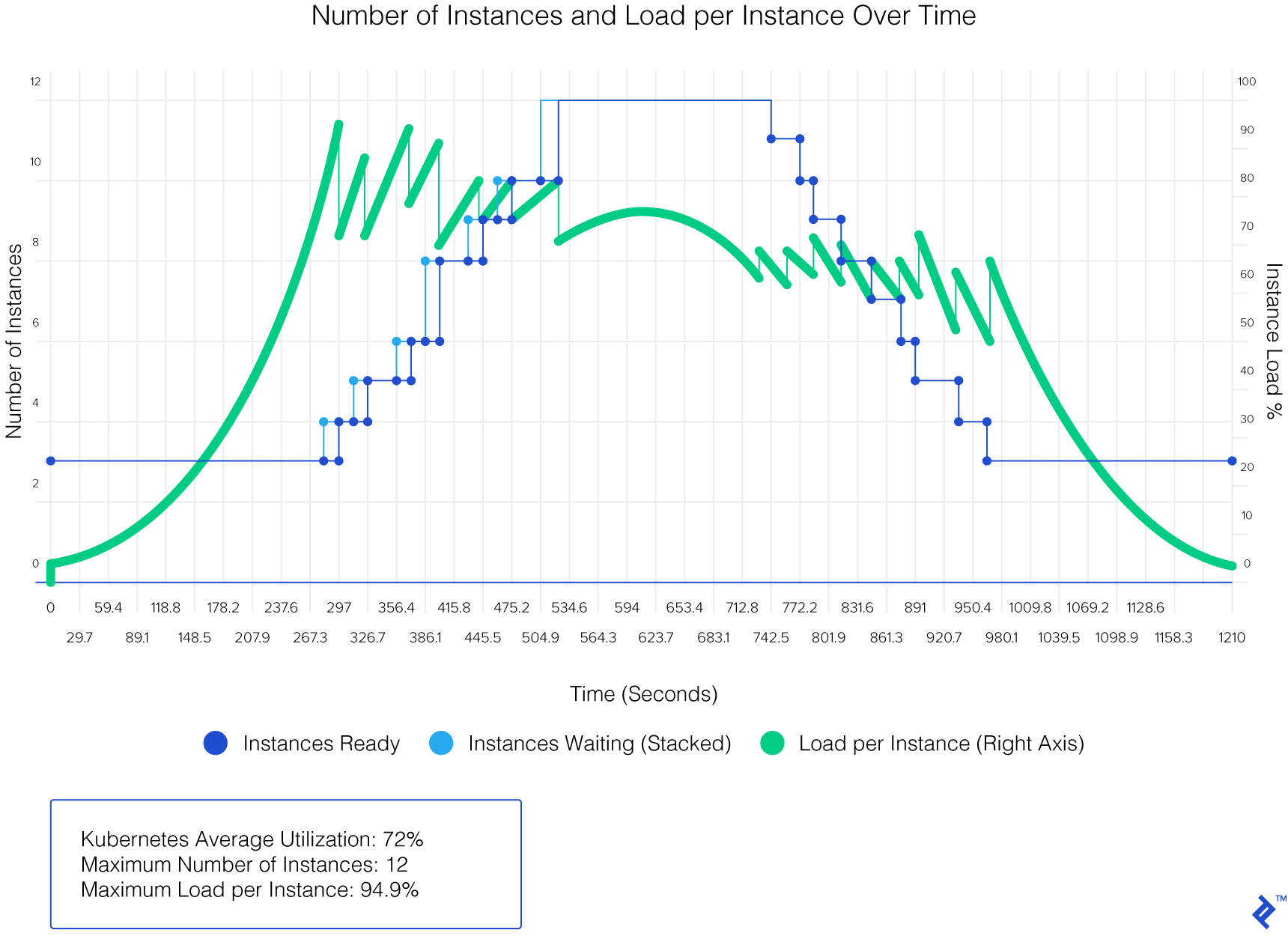
As promised, let’s delve into the web application mentioned earlier. This tool takes your load function, container orchestrator configuration, and other relevant general parameters as input, subsequently outputting the calculated scale-up threshold and other instance-related values.

The project is hosted on hosted on GitHub and can be accessed directly through a live version available.

Let’s examine the results generated by this web app using test data (on Kubernetes):

Scaling Microservices with Precision

In the realm of microservices application architectures, container deployment takes center stage. Optimal configuration of both the orchestrator and containers is paramount for a smooth and efficient runtime experience.

As DevOps practitioners, we continuously strive to refine the tuning of orchestration parameters for our applications. Let’s embrace a more mathematically-driven approach to auto-scaling microservices!