In today’s financial markets, automated trading systems, powered by sophisticated algorithms, execute over 60% of trades involving various assets like stocks, index futures, and commodities. These programs are designed to generate profits over the long term by autonomously buying and selling assets across different markets.

This article aims to demonstrate how to predict, with reasonable accuracy, the optimal trade direction to maximize gains. We’ll use the S&P 500 index, a weighted average of 500 large-cap US companies, as our trading asset. A simple strategy involves buying the index at the 9:30 AM market open and selling at the 4:00 PM close (Eastern Time). Profit or loss depends on whether the closing price is higher or lower than the opening price. This is where Machine Learning comes in – we’ll utilize its predictive power to anticipate the closing price direction.

Machine Learning is revolutionizing various fields, including finance, where it’s widely employed. The beauty of Machine Learning lies in its ability to learn patterns and relationships from data, eliminating the need for explicit programming of every rule. This learned knowledge is then used to make predictions on new, unseen data.

Disclaimer: This article focuses on demonstrating Machine Learning techniques and code examples provided are for illustrative purposes only. Not all functions are explained in detail. Replicating the provided code and tests directly is not recommended as certain details are omitted for brevity. Basic Python knowledge is assumed. While the article showcases Machine Learning’s potential in financial trading, real-world trading involves additional skills like money management and risk management, which are not covered here.

Developing Your First Financial Data Automated Trading System

Let’s build your first program for financial data analysis and trade prediction using Python and historical data from Yahoo Finance service. As mentioned, this historical data is crucial for training our predictive model.

First, ensure you have the following installed:

• Python, specifically IPython notebook.
• Yahoo Finance Python package (package name: yahoo-finance), installed via the terminal command: pip install yahoo-finance.
• A free trial of the Machine Learning package GraphLab. Refer to the documentation of that library for more details.

Note that only the SFrame component of GraphLab is open source. A license is required for full library access, with options including a 30-day free trial and a non-commercial license for students and Kaggle competitors. GraphLab Create provides an intuitive and user-friendly platform for data analysis and Machine Learning model training.

Python Code Walkthrough

Let’s dive into the Python code for downloading financial data. IPython Notebook is recommended for its integrated environment that seamlessly combines source code, execution, data tables, and charts. For a quick IPython Notebook tutorial, refer to the Introduction to IPython Notebook article.

Create a new IPython Notebook and let’s download S&P 500 historical price data. You can adapt this to your preferred IDE and create a new Python project if desired.

 1
 2
 3
 4
 5
 6
 7
 8
 9
10
11
12
13
14
15
16
17
18
19
20

import graphlab as gl
from __future__ import division
from datetime import datetime
from yahoo_finance import Share

# download historical prices of S&P 500 index
today = datetime.strftime(datetime.today(), "%Y-%m-%d")
stock = Share('^GSPC') # ^GSPC is the Yahoo finance symbol to refer S&P 500 index
# we gather historical quotes from 2001-01-01 up to today
hist_quotes = stock.get_historical('2001-01-01', today)
# here is how a row looks like
hist_quotes[0]
{'Adj_Close': '2091.580078',
 'Close': '2091.580078',
 'Date': '2016-04-22',
 'High': '2094.320068',
 'Low': '2081.199951',
 'Open': '2091.48999',
 'Symbol': '%5eGSPC',
 'Volume': '3790580000'}

The variable hist_quotes contains a list of dictionaries, each representing a trading day with attributes like Open, High, Low, Close, Adj_close, Volume, Symbol, and Date. We’ll extract relevant data, reverse the order for most recent values first, and organize it into separate lists:

 1
 2
 3
 4
 5
 6
 7
 8
 9
10
11
12
13
14
15

l_date = []
l_open = []
l_high = []
l_low = []
l_close = []
l_volume = []
# reverse the list
hist_quotes.reverse()
for quotes in hist_quotes:
    l_date.append(quotes['Date'])
    l_open.append(float(quotes['Open']))
    l_high.append(float(quotes['High']))
    l_low.append(float(quotes['Low']))
    l_close.append(float(quotes['Close']))
    l_volume.append(int(quotes['Volume']))

Next, we’ll use GraphLab’s SFrame – a scalable, compressed, disk-backed columnar data frame that can handle datasets larger than RAM – to store these quotes. Learn more about SFrame in the documentation.

Let’s store and examine our historical data:

 1
 2
 3
 4
 5
 6
 7
 8
 9
10
11

qq = gl.SFrame({'datetime' : l_date, 
          'open' : l_open, 
          'high' : l_high, 
          'low' : l_low, 
          'close' : l_close, 
          'volume' : l_volume})
# datetime is a string, so convert into datetime object
qq['datetime'] = qq['datetime'].apply(lambda x:datetime.strptime(x, '%Y-%m-%d'))

# just to check if data is sorted in ascending mode
qq.head(3)

Now, save this data to disk using the save method of the SFrame:

1
2
3

qq.save(“SP500_daily.bin”)
# once data is saved, we can use the following instruction to retrieve it 
qq = gl.SFrame(“SP500_daily.bin/”)

Visualizing the S&P 500

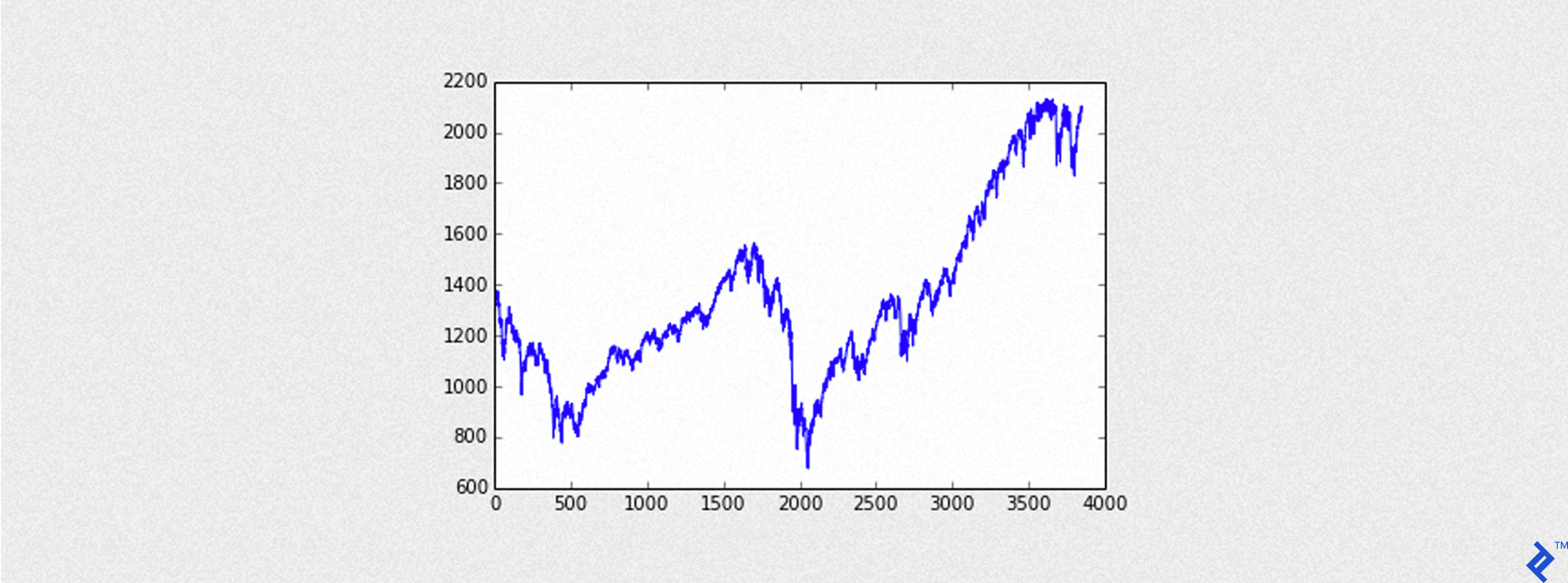
The following code visualizes the loaded S&P 500 data:

1
2
3

import matplotlib.pyplot as plt
%matplotlib inline # only for those who are using IPython notebook
plt.plot(qq['close'])

The output is a graph that looks like this:

Training Machine Learning Models

Adding the Outcome Variable

Our models aim to predict whether the closing price will exceed the opening price, indicating a potential profit opportunity. Therefore, we need to add an outcome column – our target variable – to the data. Each row in this column will have:

• +1 for an Up day (closing price higher than opening price)
• -1 for a Down day (closing price lower than opening price)

1
2
3
4
5
6
7

# add the outcome variable, 1 if the trading session was positive (close>open), 0 otherwise
qq['outcome'] = qq.apply(lambda x: 1 if x['close'] > x['open'] else -1)
# we also need to add three new columns ‘ho’ ‘lo’ and ‘gain’
# they will be useful to backtest the model, later
qq['ho'] = qq['high'] - qq['open'] # distance between Highest and Opening price
qq['lo'] = qq['low'] - qq['open'] # distance between Lowest and Opening price
qq['gain'] = qq['close'] - qq['open']

To make predictions based on past data, we’ll lag the data by one or more days using GraphLab’s TimeSeries object and its shift method:

 1
 2
 3
 4
 5
 6
 7
 8
 9
10

ts = gl.TimeSeries(qq, index='datetime')
# add the outcome variable, 1 if the bar was positive (close>open), 0 otherwise
ts['outcome'] = ts.apply(lambda x: 1 if x['close'] > x['open'] else -1)

# GENERATE SOME LAGGED TIMESERIES
ts_1 = ts.shift(1) # by 1 day
ts_2 = ts.shift(2) # by 2 days
# ...etc....
# it's an arbitrary decision how many days of lag are needed to create a good forecaster, so
# everyone can experiment by his own decision

Adding Predictors

Predictors are the features used to train our model and predict the outcome. Selecting relevant predictors is crucial for forecasting accuracy.

For example, we might consider if today’s closing price is higher than yesterday’s, and extend this to the past two days, etc. The code below illustrates this:

1
2

ts['feat1'] = ts['close'] > ts_1['close']
ts['feat2'] = ts['close'] > ts_2['close']

Here, we’ve introduced two new feature columns, feat1 and feat2, to our dataset (ts), where 1 indicates a true comparison and 0 otherwise.

This article aims to provide a practical demonstration of Machine Learning in finance. In-depth predictor selection is a complex topic and beyond our current scope. Experimenting with different factor combinations is encouraged to understand their impact on model accuracy.

 1
 2
 3
 4
 5
 6
 7
 8
 9
10
11
12
13
14
15
16

# add_features is a helper function, which is out of the scope of this article,
# and it returns a tuple with:
# ts: a timeseries object with, in addition to the already included columns, also lagged columns
# as well as some features added to train the model, as shown above with feat1 and feat2 examples
# l_features: a list with all features used to train Classifier models
# l_lr_features: a list all features used to train Linear Regression models

ts, l_features, l_lr_features = add_features(ts)

# add the gain column, for trading operations with LONG only positions. 
# The gain is the difference between Closing price - Opening price
ts['gain'] = ts['close'] - ts['open']

ratio = 0.8 # 80% of training set and 20% of testing set
training = ts.to_sframe()[0:round(len(ts)*ratio)]
testing = ts.to_sframe()[round(len(ts)*ratio):]

Training a Decision Tree Model

GraphLab Create simplifies Machine Learning model implementation. Models are trained using the create method, which takes parameters such as:

• training: The training dataset with features and the target column.
• target: Name of the target variable column.
• validation_set: Optional dataset for evaluating model generalization (not used in our case).
• features: List of feature column names for training.
• verbose: Prints training progress information if set to true.

Additional model-specific parameters can be included, such as:

• max_depth: Maximum depth of the decision tree.

Let’s build our decision tree:

1
2
3
4

max_tree_depth = 6
decision_tree = gl.decision_tree_classifier.create(training, validation_set=None, 
                                                   target='outcome', features=l_features, 
                                                   max_depth=max_tree_depth, verbose=False)

Evaluating Model Performance

Accuracy, the ratio of correct predictions to the total data points, is a key performance metric. Accuracy on the training set is typically higher than on a separate test set due to model fitting.

Precision measures the accuracy of positive predictions, and we aim for a precision closer to 1 for a high win-rate.

Recall assesses the classifier’s ability to identify positive examples, essentially the probability of correctly identifying a randomly chosen positive example. A recall closer to 1 is desirable.

GraphLab Create’s evaluate method provides these and other important model metrics.

Let’s check the model’s accuracy on both training and testing datasets:

1
2

decision_tree.evaluate(training)['accuracy'], decision_tree.evaluate(testing)['accuracy']
(0.6077348066298343, 0.577373211963589)

The test set accuracy is around 57%, slightly better than a random guess (50%).

Making Predictions

GraphLab Create uses the predict method for generating predictions from trained models. We’ll pass our testing set to predict the outcome variable.

1
2
3
4
5
6

predictions = decision_tree.predict(testing)
# and we add the predictions  column in testing set
testing['predictions'] = predictions

# let's see the first 10 predictions, compared to real values (outcome column)
testing[['datetime', 'outcome', 'predictions']].head(10)

False positives occur when the model predicts an Up Day (+1) while the actual outcome is a Down Day. Conversely, false negatives happen when the model predicts a Down Day (-1) while the actual outcome is an Up Day.

Our strategy buys the S&P 500 at the opening price when an Up Day is predicted and sells at the closing price. Minimizing false positives is crucial to avoid losses, meaning we strive for the highest possible precision.

In the first ten predictions of our test set, we observe two false negatives and two false positives.

Calculating the metrics for this small sample:

• accuracy = 6/10 = 0.6 or 60%
• precision = 3/5 = 0.6 or 60%
• recall = 3/5 = 0.6 or 60%

Note that these metrics typically differ, but they happen to be the same in this particular example.

Backtesting the Model

Let’s simulate how the model would perform in a trading scenario. A predicted outcome of +1 (Up Day) triggers a buy at the opening price and a sell at the closing price. Conversely, a predicted outcome of -1 (Down Day) results in no trade.

Profit and Loss (pnl) for each daily trade (round turn) is calculated as:

• pnl = Close - Open

The plot_equity_chart helper function (code not shown for brevity) will be used to visualize the cumulative gains (equity curve) from a series of profit and loss values.

1
2
3
4
5

pnl = testing[testing['predictions'] == 1]['gain'] # the gain column contains (Close - Open) values
# I have written a simple helper function to plot the result of all the trades applied to the
# testing set and represent the total return expressed by the index basis points
# (not expressed in dollars $)
plot_equity_chart(pnl,'Decision tree model')

1
2
3

Mean of PnL is 1.843504
Sharpe is 1.972835
Round turns 511

Here, Sharpe refers to the annualized Sharpe ratio – a crucial measure of trading strategy performance.

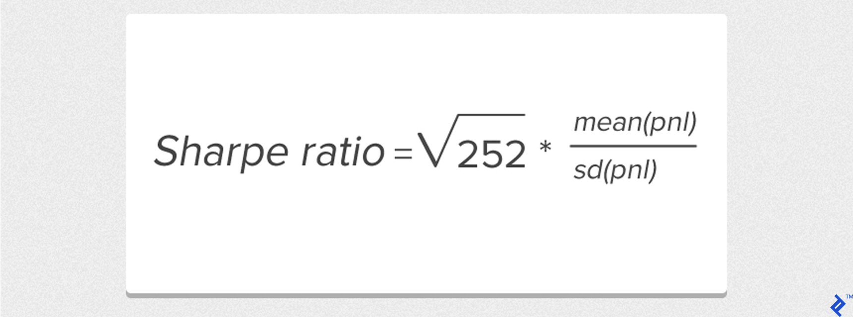
This simplified formula assumes a risk-free return of 0, with mean and sd representing the mean and standard deviation of daily profit and loss values, respectively.

Trading Fundamentals

Trading the S&P 500 requires an appropriate instrument. Many brokers offer CFDs (Contracts for Difference) – agreements to exchange the price difference between opening and closing – that track the index.

Example: Buy 1 S&P 500 CFD at the opening price of 2000 and sell at the closing price of 2020. The gain is 20 points. Assuming each point is worth $25:

• Gross Gain: 20 points x $25 = $500 for 1 CFD contract.

Factoring in a hypothetical broker slippage of 0.6 points:

• Net Gain: (20 - 0.6) points x $25 = $485.

Managing potential losses is crucial, especially with false positives where the actual closing price is lower than the opening price.

A stop-loss order limits potential losses by automatically closing the position if the asset price falls below a predetermined level.

Referring back to the Yahoo Finance data, each day has a Low price. Setting a stop-loss at -3 points from the opening price would trigger if the Low price is 5 points below the opening price (Low - Open = -5), limiting the loss to -3 points instead of -5.

Here’s a helper function to simulate trades with a stop-loss:

 1
 2
 3
 4
 5
 6
 7
 8
 9
10
11
12
13
14
15
16
17
18

# This is a helper function to trade 1 bar (for example 1 day) with a Buy order at opening session
# and a Sell order at closing session. To protect against adverse movements of the price, a STOP order
# will limit the loss to the stop level (stop parameter must be a negative number)
# each bar must contains the following attributes: 
# Open, High, Low, Close prices as well as gain = Close - Open and lo = Low - Open
def trade_with_stop(bar, slippage = 0, stop=None):
    """
    Given a bar, with a gain obtained by the closing price - opening price
    it applies a stop limit order to limit a negative loss
    If stop is equal to None, then it returns bar['gain']
    """
    bar['gain'] = bar['gain'] - slippage
    if stop<>None:
        real_stop = stop - slippage
        if bar['lo']<=stop:
            return real_stop
    # stop == None    
    return bar['gain']

Incorporating Trading Costs

Realistic backtesting requires accounting for transaction costs like broker commissions and spreads. For our simulations, we’ll use fixed costs:

• Slippage: 0.6 points
• Commission: $1 per trade ($2 per round turn)

For instance, a gross gain of 10 points (1 point = $25) would result in a net gain of (10 - 0.6) * $25 - $2 = $233 after costs.

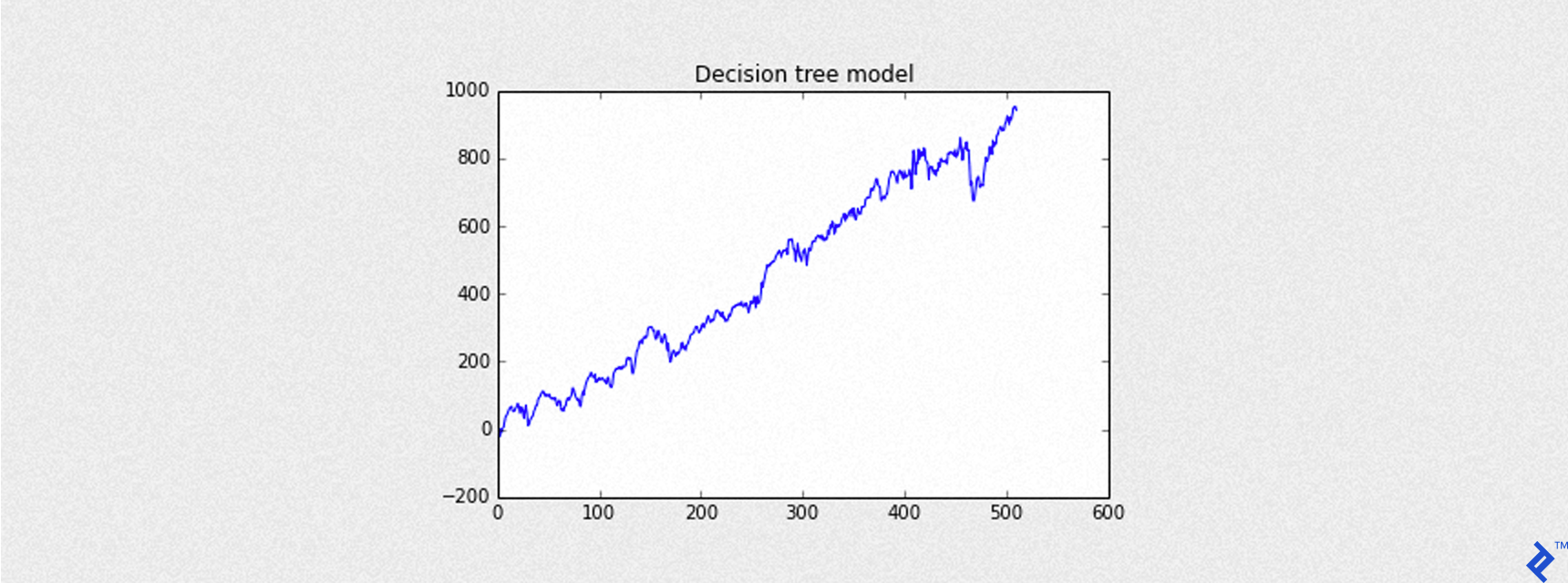
The code below simulates the trading strategy with a -3 point stop-loss. The blue line represents the equity curve (cumulative returns) considering slippage (0.6 points). Results are in basis points, consistent with the S&P 500 data.

1
2
3
4
5
6

SLIPPAGE = 0.6
STOP = -3
trades = testing[testing['predictions'] == 1][('datetime', 'gain', 'ho', 'lo', 'open', 'close')]
trades['pnl'] = trades.apply(lambda x: trade_with_stop(x, slippage=SLIPPAGE, stop=STOP))
plot_equity_chart(trades['pnl'],'Decision tree model')
print("Slippage is %s, STOP level at %s" % (SLIPPAGE, STOP))

1
2
3
4
5

Mean of PnL is 2.162171
Sharpe is 3.502897
Round turns 511
Slippage is 0.6
STOP level at -3

Let’s modify our prediction approach slightly. Instead of directly predicting the outcome class (+1 or -1), we’ll use predict(output_type="probability") to get the probability of each outcome. A probability greater than or equal to 0.5 still suggests an Up Day. Higher probabilities indicate greater confidence in the prediction.

1
2

predictions_prob = decision_tree.predict(testing, output_type = 'probability')
# predictions_prob will contain probabilities instead of the predicted class (-1 or +1)

Our updated backtesting function backtest_ml_model now considers a threshold for the predicted probability (defaulting to 0.5) to decide whether to open a trade. Trades are only opened if the predicted probability exceeds the threshold.

1

trades = testing[predictions_prob>=0.5][('datetime', 'gain', 'ho', 'lo', 'open', 'close')]

As a reminder, Net Gain for each trading day is calculated as: Net gain = (Gross gain - SLIPPAGE) * MULT - 2 * COMMISSION.

Maximum Drawdown, another vital trading strategy metric, measures the largest peak-to-trough decline in portfolio value. In our single-asset scenario, it represents the most significant drop in the equity curve.

Given an SArray of profit and loss (pnl), drawdown is calculated as:

1
2

drawdown = pnl - pnl.cumulative_max()
max_drawdown = min(drawdown)

Our backtest_summary helper function will calculate the following:

• Maximum drawdown (in dollars)
• Accuracy (using Graphlab.evaluation)
• Precision (using Graphlab.evaluation)
• Recall (using Graphlab.evaluation)

The following code demonstrates the equity curve of cumulative returns for the model, expressed in dollars.

1
2
3
4
5
6
7

model = decision_tree
predictions_prob = model.predict(testing, output_type="probability")
THRESHOLD = 0.5
bt_1_1 = backtest_ml_model(testing, predictions_prob, target='outcome',  
                           threshold=THRESHOLD, STOP=-3, 
                           MULT=25, SLIPPAGE=0.6, COMMISSION=1, plot_title='DecisionTree')
backtest_summary(bt_1_1)

1
2
3
4
5
6
7
8

Mean of PnL is 54.054286 
Sharpe is 3.502897
Round turns 511
Name: DecisionTree
Accuracy: 0.577373211964
Precision: 0.587084148728
Recall: 0.724637681159
Max Drawdown: -1769.00025

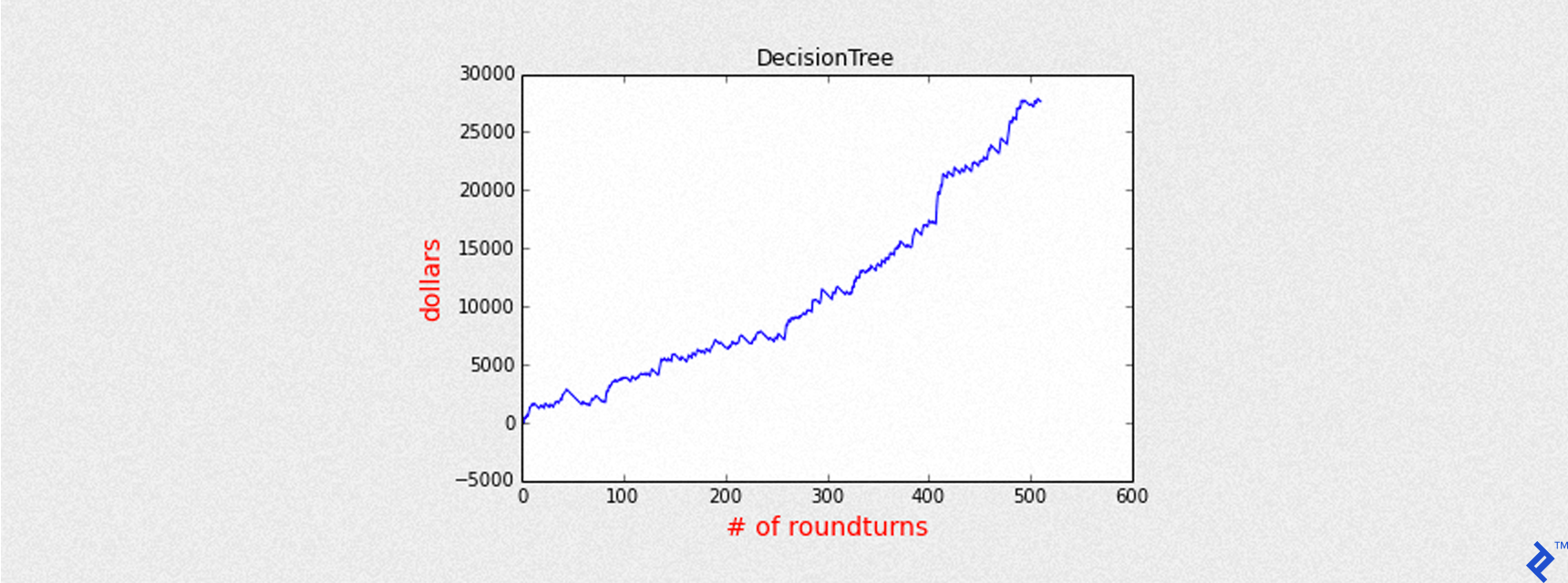
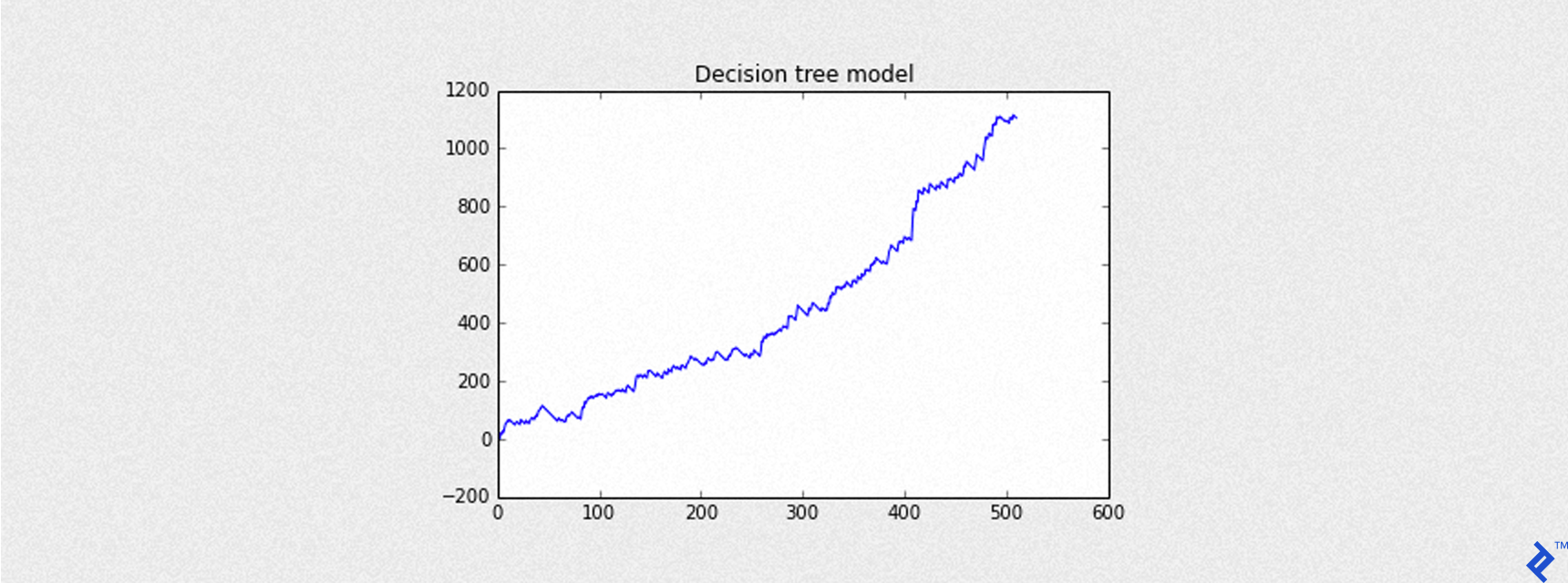
To enhance prediction precision, we can raise the threshold above 0.5, increasing our confidence in predicted Up Days.

1
2
3
4
5
6

THRESHOLD = 0.55 
# it’s the minimum threshold to predict an Up day so hopefully a good day to trade
bt_1_2 = backtest_ml_model(testing, predictions_prob, target='outcome',  
                           threshold=THRESHOLD, STOP=-3, 
                           MULT=25, SLIPPAGE=0.6, COMMISSION=1, plot_title='DecisionTree')
backtest_summary(bt_1_2)

1
2
3
4
5
6
7
8

Mean of PnL is 118.244689 
Sharpe is 6.523478
Round turns 234
Name: DecisionTree
Accuracy: 0.560468140442
Precision: 0.662393162393
Recall: 0.374396135266
Max Drawdown: -1769.00025

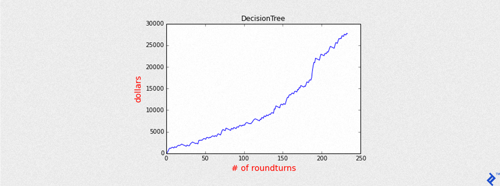
With a higher threshold, the equity curve shows considerable improvement (Sharpe ratio of 6.5 compared to 3.5 previously) despite fewer trades.

From this point onward, we’ll employ thresholds higher than 0.5 for subsequent models.

Training a Logistic Regression Model

Let’s apply our approach to a Logistic Regression model using GraphLab Create. We’ll predict probabilities instead of class labels and use a threshold above 0.5 for improved precision.

1
2
3
4
5
6
7

model = gl.logistic_classifier.create(training, target='outcome', features=l_features, 
                                      validation_set=None, verbose=False)
predictions_prob = model.predict(testing, 'probability')
THRESHOLD = 0.6
bt_2_2 = backtest_ml_model(testing, predictions_prob, target='outcome', 
                           threshold=THRESHOLD, STOP=-3, plot_title=model.name())
backtest_summary(bt_2_2)

1
2
3
4
5
6
7
8

Mean of PnL is 112.704215 
Sharpe is 6.447859
Round turns 426
Name: LogisticClassifier
Accuracy: 0.638491547464
Precision: 0.659624413146
Recall: 0.678743961353
Max Drawdown: -1769.00025

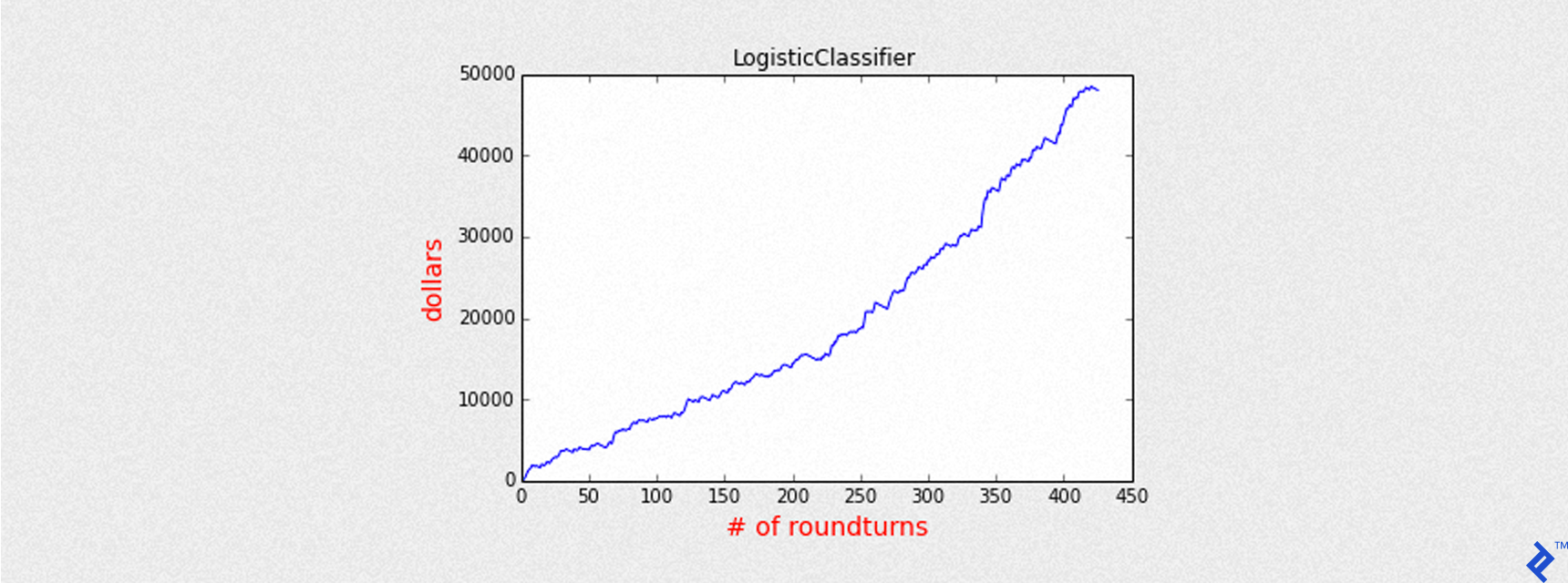
The summary output is similar to the Decision Tree model, as both are classifiers predicting binary outcomes (+1 or -1).

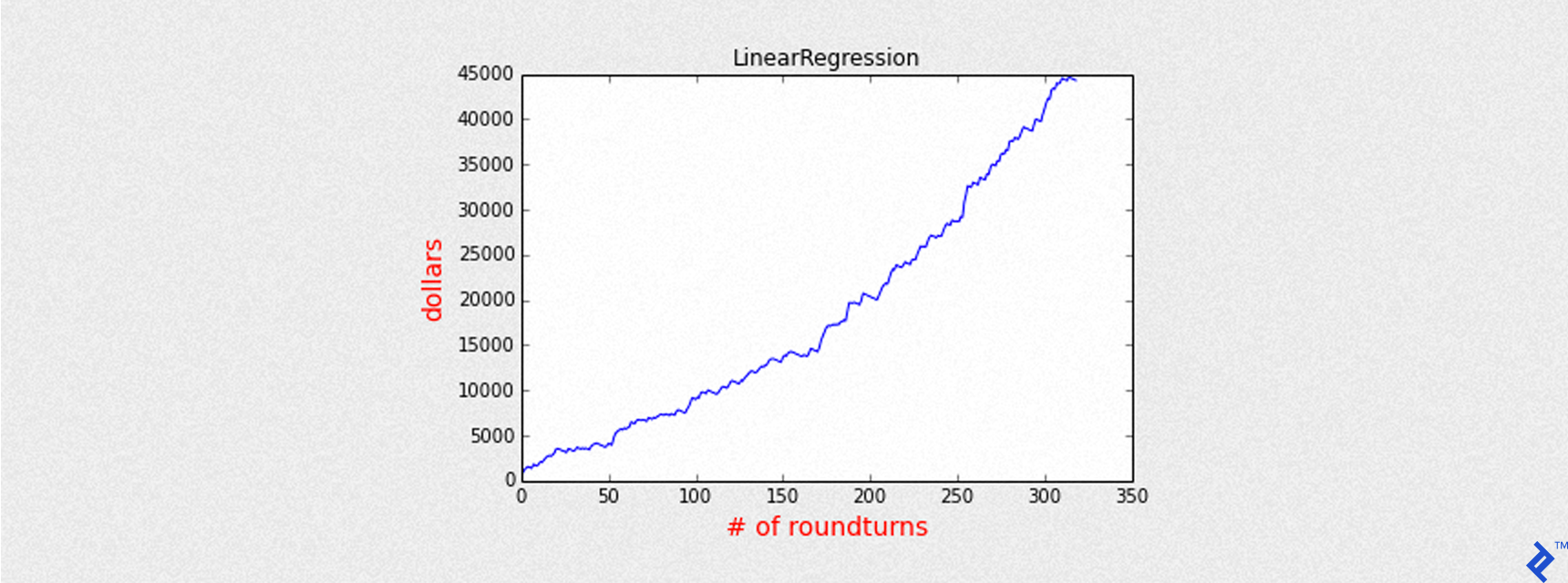
Training a Linear Regression Model

Unlike our previous classifiers, Linear Regression deals with continuous values. Instead of using +1 and -1 as target variables, we’ll use the actual gain (closing price minus opening price). Our features will also be continuous variables like previous opening and closing prices.

We won’t delve into feature selection here, focusing on applying different Machine Learning models.

Key parameters for the create method are:

• training: Training dataset with features and target variable.
• target: Name of the target variable column.
• validation_set: Optional validation dataset (not used here).
• features: List of feature columns.
• verbose: Prints training progress if true.
• max_iterations: Maximum number of passes through the data for training.

1
2
3
4
5
6
7

model = gl.linear_regression.create(training, target='gain', features = l_lr_features,
                                   validation_set=None, verbose=False, max_iterations=100)
predictions = model.predict(testing)
# a linear regression model, predict continuous values, so we need to make an estimation of their
# probabilities of success and normalize all values in order to have a vector of probabilities
predictions_max, predictions_min = max(predictions), min(predictions)
predictions_prob = (predictions - predictions_min)/(predictions_max - predictions_min)

We now have predictions (predicted gains) and predictions_prob (normalized predicted gains). A threshold of 0.4 is chosen to balance accuracy and trade frequency. The backtest_linear_model helper function only opens trades when predictions_prob exceeds this threshold.

1
2
3
4

THRESHOLD = 0.4
bt_3_2 = backtest_linear_model(testing, predictions_prob, target='gain', threshold=THRESHOLD,
                              STOP = -3, plot_title=model.name())
backtest_summary(bt_3_2)

1
2
3
4
5
6
7
8

Mean of PnL is 138.868280 
Sharpe is 7.650187
Round turns 319
Name: LinearRegression
Accuracy: 0.631989596879
Precision: 0.705329153605
Recall: 0.54347826087
Max Drawdown: -1769.00025

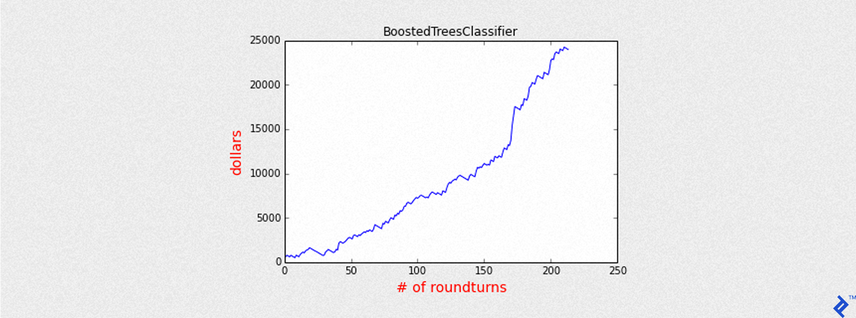
Training a Boosted Tree Model

Similar to the Decision Tree, we’ll now train a Boosted Tree Classifier. We’ll increase the max_iterations to 12 for more boosting iterations (each creating an additional tree) and use a threshold higher than 0.5 for better precision.

1
2
3
4
5
6
7
8

model = gl.boosted_trees_classifier.create(training, target='outcome', features=l_features, 
                                           validation_set=None, max_iterations=12, verbose=False)
predictions_prob = model.predict(testing, 'probability')

THRESHOLD = 0.7
bt_4_2 = backtest_ml_model(testing, predictions_prob, target='outcome', 
                           threshold=THRESHOLD, STOP=-3, plot_title=model.name())
backtest_summary(bt_4_2)

1
2
3
4
5
6
7
8

Mean of PnL is 112.002338
Sharpe is 6.341981
Round turns 214
Name: BoostedTreesClassifier
Accuracy: 0.563068920676
Precision: 0.682242990654
Recall: 0.352657004831
Max Drawdown: -1769.00025

Training a Random Forest Model

Finally, let’s train a Random Forest Classifier – an ensemble of decision trees. We’ll limit the number of trees to num_trees = 10 to manage complexity and prevent overfitting.

1
2
3
4
5
6
7

model = gl.random_forest_classifier.create(training, target='outcome', features=l_features, 
                                      validation_set=None, verbose=False, num_trees = 10)
predictions_prob = model.predict(testing, 'probability')
THRESHOLD = 0.6
bt_5_2 = backtest_ml_model(testing, predictions_prob, target='outcome', 
                           threshold=THRESHOLD, STOP=-3, plot_title=model.name())
backtest_summary(bt_5_2)

1
2
3
4
5
6
7
8

Mean of PnL is 114.786962 
sharpe is 6.384243
Round turns 311
Name: RandomForestClassifier
Accuracy: 0.598179453836
Precision: 0.668810289389
Recall: 0.502415458937
Max Drawdown: -1769.00025

Combining All Models

Now, let’s analyze the collective performance of all our models, sorted by precision.

By aggregating the daily profit and loss from each model (pnl), we can visualize the combined equity curve.

1
2
3
4
5
6

Mean of PnL is 119.446463
Sharpe is 6.685744
Round turns 1504
First trading day 2013-04-09
Last trading day 2016-04-22 
Total return 179647

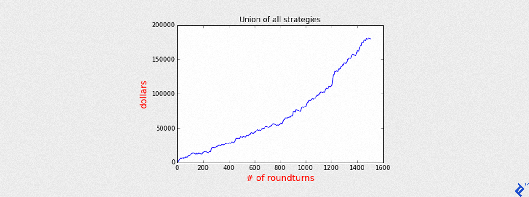
Over approximately 3 years of simulated trading, the combined models generate a total gain of roughly $180,000. The maximum exposure is 5 CFD contracts, closed at the end of each day to avoid overnight positions.

Analyzing the Aggregated Model Performance

Since we have 5 models running concurrently, the number of open trades on a given day can range from 1 to 5. We can group trades by the number of models agreeing on an Up Day and analyze precision accordingly.

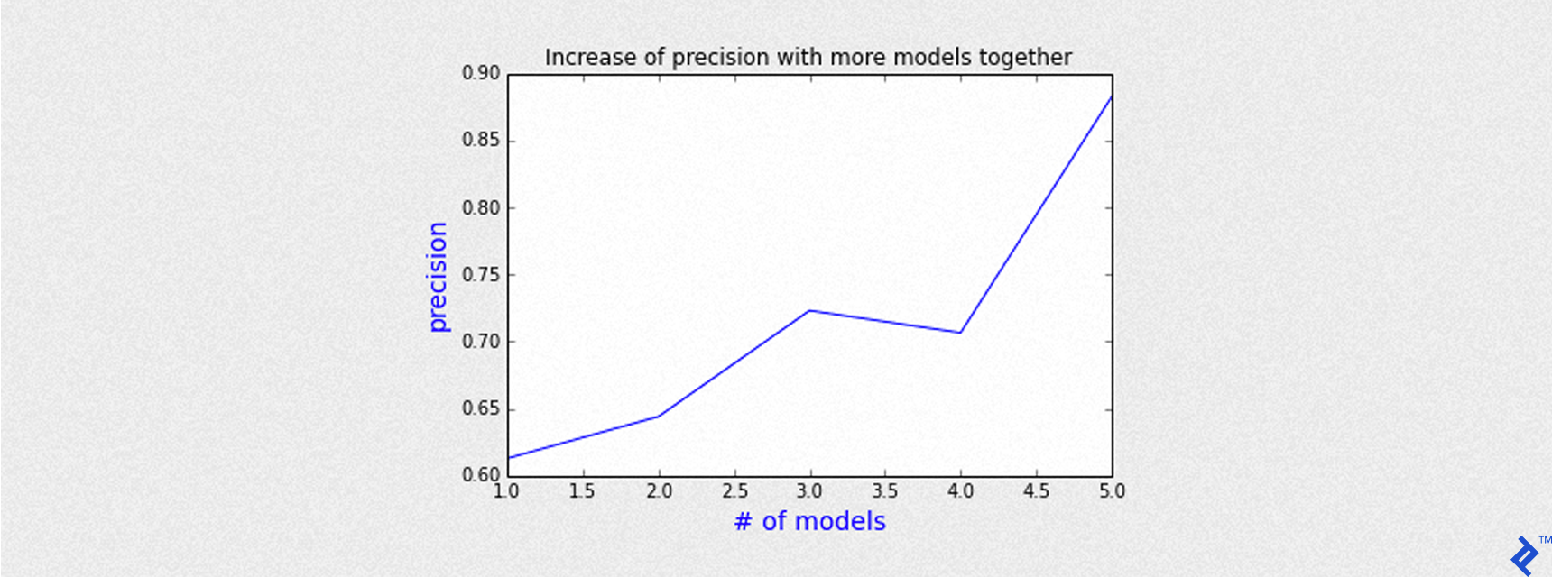
The chart above demonstrates that precision increases with the number of agreeing models. For example, when all 5 models predict an Up Day, the precision surpasses 85%.

Conclusion

Machine Learning offers powerful tools for learning from data and generating valuable predictions, even in the complex world of finance. While individual model performance varies, combining multiple models can lead to superior results. GraphLab Create provides an efficient and scalable platform for handling Big Data and implementing various scientific and forecasting models. Its free licensing options for students and Kaggle participants make it an accessible choice for exploration and learning.

Important Note: This article is intended for informational purposes only and should not be considered financial advice. Examples provided are for educational purposes only. Past performance is not indicative of future results. Always consult with a qualified financial advisor before making any investment decisions.