Bioinformatics involves creating methods and software to help us understand biological data.
It’s like data science, but for biology.
Genomics data, especially from next-generation DNA sequencing (NGS), is increasing rapidly. Stephens, Zachary D et al. shows that we’re now gathering genomics data at an exabyte-per-year rate.
SciPy gathers many Python modules for scientific computing, which is ideal for many bioinformatic needs.
This post demonstrates how to analyze human genome data in a GFF3 file using the SciPy Stack. The Generic Feature Format Version 3 (GFF3) is the standard format for storing genomic features. This post will show you how to use SciPy to answer these questions:
- How much of the human genome is incomplete?
- How many genes are in the human genome?
- What is the average size of a gene?
- How are genes distributed among chromosomes?
You can get the latest human genome GFF3 file from here. The README. This directory also includes a file explaining the GFF3 format, and you can find a complete specification here.
We’ll use Pandas, a powerful SciPy tool, to work with the GFF3 data.
Setting Up
First, we’ll set up a virtual environment and install SciPy. This can take a while if done manually because SciPy has many packages. Using Miniconda simplifies the process.
1
2
| wget https://repo.continuum.io/miniconda/Miniconda3-latest-Linux-x86_64.sh
bash Miniconda3-latest-Linux-x86_64.sh -b
|
The -b flag tells bash to run in batch mode. After installing Miniconda, create a virtual environment for genomics and install SciPy.
1
2
3
| mkdir -p genomics
cd genomics
conda create -p venv ipython matplotlib pandas
|
This installs the three packages needed for this post. You can add more SciPy packages to the conda create command.
Use conda search to find package names. Now, activate the virtual environment and start IPython.
1
2
| source activate venv/
ipython
|
IPython is a more powerful alternative to the standard Python interpreter. Anything you do in the default interpreter, you can do in IPython. If you haven’t tried it, I highly recommend it.
Downloading the Annotation File
Now that we’re set up, let’s download the human genome annotation (GFF3 format).
It’s around 37 MB, much smaller than the entire human genome (about 3 GB in plain text). That’s because it only contains annotations, while the actual sequence data is stored in the FASTA format. You can download the FASTA file here, but we won’t be using it in this tutorial.
1
| !wget ftp://ftp.ensembl.org/pub/release-85/gff3/homo_sapiens/Homo_sapiens.GRCh38.85.gff3.gz
|
The ! tells IPython that this is a shell command, not a Python command. However, IPython can process common shell commands like ls, pwd, rm, mkdir, and rmdir without the !.
Looking at the beginning of the GFF file, you’ll see lines starting with ## or #! containing metadata/pragmas/directives.
According to the README, ## indicates stable metadata, while #! indicates experimental metadata.
You’ll also see ###, which has a more specific meaning defined in the specification.
Comments meant for humans appear after a single #. For this analysis, we’ll ignore all lines starting with #.
 1
 2
 3
 4
 5
 6
 7
 8
 9
10
11
12
13
14
| ##gff-version 3
##sequence-region 1 1 248956422
##sequence-region 10 1 133797422
##sequence-region 11 1 135086622
##sequence-region 12 1 133275309
...
##sequence-region MT 1 16569
##sequence-region X 1 156040895
##sequence-region Y 2781480 56887902
#!genome-build GRCh38.p7
#!genome-version GRCh38
#!genome-date 2013-12
#!genome-build-accession NCBI:GCA_000001405.22
#!genebuild-last-updated 2016-06
|
The first line indicates that the file uses GFF version 3.
Following that are summaries of all sequence regions, which are also found later in the file.
Lines beginning with #! provide information about the specific genome build this annotation file corresponds to, which is GRCh38.p7.
The Genome Reference Consortium (GCR) is an international group that manages updates to reference genome assemblies for various species, including humans, mice, zebrafish, and chickens.
Here are the first few annotation lines in the file:
1
2
3
4
5
6
7
8
| 1 GRCh38 chromosome 1 248956422 . . . ID=chromosome:1;Alias=CM000663.2,chr1,NC_000001.11
###
1 . biological_region 10469 11240 1.3e+03 . . external_name=oe %3D 0.79;logic_name=cpg
1 . biological_region 10650 10657 0.999 + . logic_name=eponine
1 . biological_region 10655 10657 0.999 - . logic_name=eponine
1 . biological_region 10678 10687 0.999 + . logic_name=eponine
1 . biological_region 10681 10688 0.999 - . logic_name=eponine
...
|
The columns are seqid, source, type, start, end, score, strand, phase, attributes. Some are self-explanatory. For example:
1
| 1 GRCh38 chromosome 1 248956422 . . . ID=chromosome:1;Alias=CM000663.2,chr1,NC_000001.11
|
This line represents the first chromosome, with a seqid of 1. It starts at the first base and extends to the 24,895,622nd base, meaning the chromosome is about 25 million bases long.
Our analysis won’t use the score, strand, and phase columns, so we can ignore them. The attributes column tells us that Chromosome 1 has three aliases: CM000663.2, chr1, and NC_000001.11. That’s the basic structure of a GFF3 file. We won’t examine every line; instead, let’s load the whole file into Pandas.
Pandas is ideal for working with GFF3 files because they are tab-delimited, and Pandas excels at handling CSV-like formats.
One exception is when the GFF3 file contains ##FASTA.
As explained in the specification, ##FASTA marks the end of an annotation section and the beginning of one or more sequences in FASTA format (which is not tab-delimited). However, our GFF3 file doesn’t have this.
 1
 2
 3
 4
 5
 6
 7
 8
 9
10
11
| In [1]: import pandas as pd
In [2]: pd.__version__
Out[2]: '0.18.1'
In [3]: col_names = ['seqid', 'source', 'type', 'start', 'end', 'score', 'strand', 'phase', 'attributes']
Out[3]: df = pd.read_csv('Homo_sapiens.GRCh38.85.gff3.gz', compression='gzip',
sep='\t', comment='#', low_memory=False,
header=None, names=col_names)
|
This code snippet uses pandas.read_csv to load the GFF3 file.
Since it’s not a standard CSV, we need some adjustments.
header=None tells Pandas that the file lacks a header.
names=col_names assigns specific names to each column. Without this, Pandas would use numbers.
sep='\t' indicates that tabs separate the columns, not commas. You can use regular expressions (regex) for more complex separators. comment='#' tells Pandas to ignore lines starting with #.
compression='gzip' specifies that the file is gzip-compressed.
pandas.read_csv offers many options for reading different CSV-like formats.
The result is a DataFrame, Pandas’s primary data structure for representing 2D data.
Pandas also provides Series and Panel for 1D and 3D data, respectively. The documentation introduces Pandas’s data structures.
Let’s view the first few entries with .head:
1
2
3
4
5
6
7
8
| In [18]: df.head()
Out[18]:
seqid source type start end score strand phase attributes
0 1 GRCh38 chromosome 1 248956422 . . . ID=chromosome:1;Alias=CM000663.2,chr1,NC_00000...
1 1 . biological_region 10469 11240 1.3e+03 . . external_name=oe %3D 0.79;logic_name=cpg
2 1 . biological_region 10650 10657 0.999 + . logic_name=eponine
3 1 . biological_region 10655 10657 0.999 - . logic_name=eponine
4 1 . biological_region 10678 10687 0.999 + . logic_name=eponine
|
The output is neatly formatted, with long strings in the attributes column truncated and replaced with ....
To display full strings, use pd.set_option('display.max_colwidth', -1). Pandas offers many customizable options.
Now, let’s get basic information about the dataframe with .info:
 1
 2
 3
 4
 5
 6
 7
 8
 9
10
11
12
13
14
15
| In [20]: df.info()
<class 'pandas.core.frame.DataFrame'>
RangeIndex: 2601849 entries, 0 to 2601848
Data columns (total 9 columns):
seqid object
source object
type object
start int64
end int64
score object
strand object
phase object
attributes object
dtypes: int64(2), object(7)
memory usage: 178.7+ MB
|
This tells us that the GFF3 file has 2,601,848 lines, each with nine columns.
We also see the data type for each column.
Start and end are integers (int64) representing genome positions.
Other columns have the object type, meaning they likely contain a mix of integers, floats, and strings.
The data occupies 178.7+ MB of memory, making it more compact than the uncompressed file (around 402 MB), as confirmed below:
1
2
| gunzip -c Homo_sapiens.GRCh38.85.gff3.gz > /tmp/tmp.gff3 && du -s /tmp/tmp.gff3
402M /tmp/tmp.gff3
|
We’ve loaded the entire GFF3 file into a Python DataFrame. All subsequent analysis will be based on this object.
Let’s examine the first column, seqid.
1
2
3
4
5
6
7
8
9
| In [29]: df.seqid.unique()
Out[29]:
array(['1', '10', '11', '12', '13', '14', '15', '16', '17', '18', '19',
'2', '20', '21', '22', '3', '4', '5', '6', '7', '8', '9',
'GL000008.2', 'GL000009.2', 'GL000194.1', 'GL000195.1',
...
'KI270757.1', 'MT', 'X', 'Y'], dtype=object)
In [30]: df.seqid.unique().shape
Out[30]: (194,)
|
Accessing column data in a dataframe can be done with df.seqid or df['seqid']. The latter is more versatile, especially when column names are Python keywords (like class) or contain periods or spaces.
The output shows 194 unique seqids: Chromosomes 1 to 22, X, Y, mitochondrion (MT) DNA, and 169 others.
Seqids starting with KI and GL are DNA segments – or scaffolds – that haven’t been assembled into chromosomes.
This is a crucial point in genomics. While the first draft of the human genome was published over 15 years ago, it remains incomplete. Assembling these sequences is challenging, largely due to complex repetitive regions in the genome.
Now, let’s look at the source column.
The README file explains that the source describes the algorithm or process that generated the feature.
1
2
3
4
5
6
7
8
9
| In [66]: df.source.value_counts()
Out[66]:
havana 1441093
ensembl_havana 745065
ensembl 228212
. 182510
mirbase 4701
GRCh38 194
insdc 74
|
This demonstrates the value_counts method, invaluable for quickly counting categorical variables.
We see seven unique values in this column. Most GFF3 entries originate from havana, ensembl, and ensembl_havana.
You can delve deeper into these sources and their relationships in this post.
For simplicity, we’ll focus on entries from GRCh38, havana, ensembl, and ensembl_havan.a.
How Much of the Genome Is Incomplete?
Entries from source GRCh38 contain information about each chromosome. Let’s filter out the rest and store the result in a new variable, gdf.
 1
 2
 3
 4
 5
 6
 7
 8
 9
10
11
12
13
14
15
16
| In [70]: gdf = df[df.source == 'GRCh38']
In [87]: gdf.shape
Out[87]: (194, 9)
In [84]: gdf.sample(10)
Out[84]:
seqid source type start end score strand phase attributes
2511585 KI270708.1 GRCh38 supercontig 1 127682 . . . ID=supercontig:KI270708.1;Alias=chr1_KI270708v...
2510840 GL000208.1 GRCh38 supercontig 1 92689 . . . ID=supercontig:GL000208.1;Alias=chr5_GL000208v...
990810 17 GRCh38 chromosome 1 83257441 . . . ID=chromosome:17;Alias=CM000679.2,chr17,NC_000...
2511481 KI270373.1 GRCh38 supercontig 1 1451 . . . ID=supercontig:KI270373.1;Alias=chrUn_KI270373...
2511490 KI270384.1 GRCh38 supercontig 1 1658 . . . ID=supercontig:KI270384.1;Alias=chrUn_KI270384...
2080148 6 GRCh38 chromosome 1 170805979 . . . ID=chromosome:6;Alias=CM000668.2,chr6,NC_00000...
2511504 KI270412.1 GRCh38 supercontig 1 1179 . . . ID=supercontig:KI270412.1;Alias=chrUn_KI270412...
1201561 19 GRCh38 chromosome 1 58617616 . . . ID=chromosome:19;Alias=CM000681.2,chr19,NC_000...
2511474 KI270340.1 GRCh38 supercontig 1 1428 . . . ID=supercontig:KI270340.1;Alias=chrUn_KI270340...
2594560 Y GRCh38 chromosome 2781480 56887902 . . . ID=chromosome:Y;Alias=CM000686.2,chrY,NC_00002...
|
Filtering is straightforward in Pandas.
The expression df.source == 'GRCh38' generates a series of True and False values for each entry, aligned with df’s index. Using this in df[] selects only entries with a corresponding True value.
There are 194 keys in df[] where df.source == 'GRCh38'.
Since there are 194 unique seqids, each entry in gdf represents a specific seqid.
We randomly choose 10 entries with the sample method for examination.
Unassembled sequences have a type of supercontig, while others are classified as chromosomes. To calculate the proportion of the genome that’s incomplete, we need the total genome length (the sum of all seqid lengths).
 1
 2
 3
 4
 5
 6
 7
 8
 9
10
11
12
13
14
15
| In [90]: gdf = gdf.copy()
In [91]: gdf['length'] = gdf.end - gdf.start + 1
In [93]: gdf.head()
Out[93]:
seqid source type start end score strand phase attributes length
0 1 GRCh38 chromosome 1 248956422 . . . ID=chromosome:1;Alias=CM000663.2,chr1,NC_00000... 248956421
235068 10 GRCh38 chromosome 1 133797422 . . . ID=chromosome:10;Alias=CM000672.2,chr10,NC_000... 133797421
328938 11 GRCh38 chromosome 1 135086622 . . . ID=chromosome:11;Alias=CM000673.2,chr11,NC_000... 135086621
483370 12 GRCh38 chromosome 1 133275309 . . . ID=chromosome:12;Alias=CM000674.2,chr12,NC_000... 133275308
634486 13 GRCh38 chromosome 1 114364328 . . . ID=chromosome:13;Alias=CM000675.2,chr13,NC_000... 114364327
In [97]: gdf.length.sum()
Out[97]: 3096629532
In [99]: chrs = [str(_) for _ in range(1, 23)] + ['X', 'Y', 'MT']
In [101]: gdf[-gdf.seqid.isin(chrs)].length.sum() / gdf.length.sum()
Out[101]: 0.0037021917421198327
|
First, we create a copy of gdf with .copy(). Directly modifying a slice of df would trigger a SettingWithCopyWarning (see here for more details).
We calculate each entry’s length and add it to gdf as a new column called “length”. The total length is roughly 3.1 billion bases, with unassembled sequences constituting about 0.37%.
Here’s how slicing works in the last two commands.
We create a list, chrs, containing all well-assembled sequences (chromosomes and mitochondria). We use the isin method to filter for entries whose seqid is in chrs.
The minus sign (-) before the index reverses the selection, keeping entries not in the list (the unassembled sequences starting with KI and GL).
Note: We could also filter by the type column to achieve the same result:
1
| gdf[(gdf['type'] == 'supercontig')].length.sum() / gdf.length.sum()
|
How Many Genes Are There?
Now, we’ll focus on entries from sources ensembl, havana, and ensembl_havana, which contain most annotation entries.
 1
 2
 3
 4
 5
 6
 7
 8
 9
10
11
12
13
14
15
16
17
18
19
20
21
22
23
24
25
| In [109]: edf = df[df.source.isin(['ensembl', 'havana', 'ensembl_havana'])]
In [111]: edf.sample(10)
Out[111]:
seqid source type start end score strand phase attributes
915996 16 havana CDS 27463541 27463592 . - 2 ID=CDS:ENSP00000457449;Parent=transcript:ENST0...
2531429 X havana exon 41196251 41196359 . + . Parent=transcript:ENST00000462850;Name=ENSE000...
1221944 19 ensembl_havana CDS 5641740 5641946 . + 0 ID=CDS:ENSP00000467423;Parent=transcript:ENST0...
243070 10 havana exon 13116267 13116340 . + . Parent=transcript:ENST00000378764;Name=ENSE000...
2413583 8 ensembl_havana exon 144359184 144359423 . + . Parent=transcript:ENST00000530047;Name=ENSE000...
2160496 6 havana exon 111322569 111322678 . - . Parent=transcript:ENST00000434009;Name=ENSE000...
839952 15 havana exon 76227713 76227897 . - . Parent=transcript:ENST00000565910;Name=ENSE000...
957782 16 ensembl_havana exon 67541653 67541782 . + . Parent=transcript:ENST00000379312;Name=ENSE000...
1632979 21 ensembl_havana exon 37840658 37840709 . - . Parent=transcript:ENST00000609713;Name=ENSE000...
1953399 4 havana exon 165464390 165464586 . + . Parent=transcript:ENST00000511992;Name=ENSE000...
In [123]: edf.type.value_counts()
Out[123]:
exon 1180596
CDS 704604
five_prime_UTR 142387
three_prime_UTR 133938
transcript 96375
gene 42470
processed_transcript 28228
...
Name: type, dtype: int64
|
Again, we use isin for filtering.
A quick value count reveals that most entries are exons, coding sequences (CDS), and untranslated regions (UTR). These are sub-gene elements.
We see 42,470 genes, but let’s dig deeper. What are their names and functions? This information is in the attributes column.
 1
 2
 3
 4
 5
 6
 7
 8
 9
10
11
12
13
14
| In [127]: ndf = edf[edf.type == 'gene']
In [173]: ndf = ndf.copy()
In [133]: ndf.sample(10).attributes.values
Out[133]:
array(['ID=gene:ENSG00000228611;Name=HNF4GP1;biotype=processed_pseudogene;description=hepatocyte nuclear factor 4 gamma pseudogene 1 [Source:HGNC Symbol%3BAcc:HGNC:35417];gene_id=ENSG00000228611;havana_gene=OTTHUMG00000016986;havana_version=2;logic_name=havana;version=2',
'ID=gene:ENSG00000177189;Name=RPS6KA3;biotype=protein_coding;description=ribosomal protein S6 kinase A3 [Source:HGNC Symbol%3BAcc:HGNC:10432];gene_id=ENSG00000177189;havana_gene=OTTHUMG00000021231;havana_version=5;logic_name=ensembl_havana_gene;version=12',
'ID=gene:ENSG00000231748;Name=RP11-227H15.5;biotype=antisense;gene_id=ENSG00000231748;havana_gene=OTTHUMG00000018373;havana_version=1;logic_name=havana;version=1',
'ID=gene:ENSG00000227426;Name=VN1R33P;biotype=unitary_pseudogene;description=vomeronasal 1 receptor 33 pseudogene [Source:HGNC Symbol%3BAcc:HGNC:37353];gene_id=ENSG00000227426;havana_gene=OTTHUMG00000154474;havana_version=1;logic_name=havana;version=1',
'ID=gene:ENSG00000087250;Name=MT3;biotype=protein_coding;description=metallothionein 3 [Source:HGNC Symbol%3BAcc:HGNC:7408];gene_id=ENSG00000087250;havana_gene=OTTHUMG00000133282;havana_version=3;logic_name=ensembl_havana_gene;version=8',
'ID=gene:ENSG00000177108;Name=ZDHHC22;biotype=protein_coding;description=zinc finger DHHC-type containing 22 [Source:HGNC Symbol%3BAcc:HGNC:20106];gene_id=ENSG00000177108;havana_gene=OTTHUMG00000171575;havana_version=3;logic_name=ensembl_havana_gene;version=5',
'ID=gene:ENSG00000249784;Name=SCARNA22;biotype=scaRNA;description=small Cajal body-specific RNA 22 [Source:HGNC Symbol%3BAcc:HGNC:32580];gene_id=ENSG00000249784;logic_name=ncrna;version=1',
'ID=gene:ENSG00000079101;Name=CLUL1;biotype=protein_coding;description=clusterin like 1 [Source:HGNC Symbol%3BAcc:HGNC:2096];gene_id=ENSG00000079101;havana_gene=OTTHUMG00000178252;havana_version=7;logic_name=ensembl_havana_gene;version=16',
'ID=gene:ENSG00000229224;Name=AC105398.3;biotype=antisense;gene_id=ENSG00000229224;havana_gene=OTTHUMG00000152025;havana_version=1;logic_name=havana;version=1',
'ID=gene:ENSG00000255552;Name=LY6G6E;biotype=protein_coding;description=lymphocyte antigen 6 complex%2C locus G6E (pseudogene) [Source:HGNC Symbol%3BAcc:HGNC:13934];gene_id=ENSG00000255552;havana_gene=OTTHUMG00000166419;havana_version=1;logic_name=ensembl_havana_gene;version=7'], dtype=object)
|
This column contains semicolon-separated tag-value pairs. We’ll extract gene names, IDs, and descriptions using regular expressions.
 1
 2
 3
 4
 5
 6
 7
 8
 9
10
| import re
RE_GENE_NAME = re.compile(r'Name=(?P<gene_name>.+?);')
def extract_gene_name(attributes_str):
res = RE_GENE_NAME.search(attributes_str)
return res.group('gene_name')
ndf['gene_name'] = ndf.attributes.apply(extract_gene_name)
|
First, we extract gene names.
In the regex Name=(?P<gene_name>.+?); , +? ensures a non-greedy match, stopping at the first semicolon. Otherwise, it would match up to the last semicolon.
We compile the regex with re.compile for efficiency, as we’ll apply it to many attribute strings.
extract_gene_name is a helper function used with pd.apply, which applies a function to each DataFrame or Series entry.
In this case, we extract the gene name for each entry in ndf.attributes and add it to ndf as a new column called gene_name.
Gene IDs and descriptions are extracted similarly.
 1
 2
 3
 4
 5
 6
 7
 8
 9
10
11
12
13
14
15
16
17
18
19
| RE_GENE_ID = re.compile(r'gene_id=(?P<gene_id>ENSG.+?);')
def extract_gene_id(attributes_str):
res = RE_GENE_ID.search(attributes_str)
return res.group('gene_id')
ndf['gene_id'] = ndf.attributes.apply(extract_gene_id)
RE_DESC = re.compile('description=(?P<desc>.+?);')
def extract_description(attributes_str):
res = RE_DESC.search(attributes_str)
if res is None:
return ''
else:
return res.group('desc')
ndf['desc'] = ndf.attributes.apply(extract_description)
|
RE_GENE_ID is more specific, as every gene_id must start with ENSG, where ENS represents ensembl and G stands for gene.
We return an empty string for entries without a description. As we won’t need the attributes column anymore, let’s remove it with .drop:
1
2
3
4
5
6
7
8
9
| In [224]: ndf.drop('attributes', axis=1, inplace=True)
In [225]: ndf.head()
Out[225]:
seqid source type start end score strand phase gene_id gene_name desc
16 1 havana gene 11869 14409 . + . ENSG00000223972 DDX11L1 DEAD/H-box helicase 11 like 1 [Source:HGNC Sym...
28 1 havana gene 14404 29570 . - . ENSG00000227232 WASH7P WAS protein family homolog 7 pseudogene [Sourc...
71 1 havana gene 52473 53312 . + . ENSG00000268020 OR4G4P olfactory receptor family 4 subfamily G member...
74 1 havana gene 62948 63887 . + . ENSG00000240361 OR4G11P olfactory receptor family 4 subfamily G member...
77 1 ensembl_havana gene 69091 70008 . + . ENSG00000186092 OR4F5 olfactory receptor family 4 subfamily F member...
|
Here, attributes specifies the column to drop.
axis=1 indicates column removal (the default is axis=0 for rows).
inplace=True modifies the DataFrame directly instead of creating a copy.
A quick .head check confirms that the attributes column is gone, replaced by gene_name, gene_id, and desc.
Out of curiosity, let’s see if gene_id and gene_name are unique:
1
2
3
4
5
6
| In [232]: ndf.shape
Out[232]: (42470, 11)
In [233]: ndf.gene_id.unique().shape
Out[233]: (42470,)
In [234]: ndf.gene_name.unique().shape
Out[234]: (42387,)
|
There are fewer gene names than gene IDs, implying that some gene names are associated with multiple gene IDs. Let’s find them.
 1
 2
 3
 4
 5
 6
 7
 8
 9
10
11
12
13
14
15
16
17
18
19
20
21
| In [243]: count_df = ndf.groupby('gene_name').count().ix[:, 0].sort_values().ix[::-1]
In [244]: count_df.head(10)
Out[244]:
gene_name
SCARNA20 7
SCARNA16 6
SCARNA17 5
SCARNA15 4
SCARNA21 4
SCARNA11 4
Clostridiales-1 3
SCARNA4 3
C1QTNF9B-AS1 2
C11orf71 2
Name: seqid, dtype: int64
In [262]: count_df[count_df > 1].shape
Out[262]: (63,)
In [263]: count_df.shape
Out[263]: (42387,)
In [264]: count_df[count_df > 1].shape[0] / count_df.shape[0]
Out[264]: 0.0014863047632528842
|
We group entries by gene_name and count the items in each group with .count().
Inspecting the output of ndf.groupby('gene_name').count() shows that all columns are counted for each group, but most have the same value.
Note that NA values are excluded from the count. We only need the count from the first column, seqid, which has no NA values (ensured by .ix[:, 0]).
We then sort the counts using .sort_values and reverse the order with .ix[::-1].
The result shows that a gene name can be shared by up to seven gene IDs.
 1
 2
 3
 4
 5
 6
 7
 8
 9
10
| In [255]: ndf[ndf.gene_name == 'SCARNA20']
Out[255]:
seqid source type start end score strand phase gene_id gene_name desc
179399 1 ensembl gene 171768070 171768175 . + . ENSG00000253060 SCARNA20 Small Cajal body specific RNA 20 [Source:RFAM%3BAcc:RF00601]
201037 1 ensembl gene 204727991 204728106 . + . ENSG00000251861 SCARNA20 Small Cajal body specific RNA 20 [Source:RFAM%3BAcc:RF00601]
349203 11 ensembl gene 8555016 8555146 . + . ENSG00000252778 SCARNA20 Small Cajal body specific RNA 20 [Source:RFAM%3BAcc:RF00601]
718520 14 ensembl gene 63479272 63479413 . + . ENSG00000252800 SCARNA20 Small Cajal body specific RNA 20 [Source:RFAM%3BAcc:RF00601]
837233 15 ensembl gene 75121536 75121666 . - . ENSG00000252722 SCARNA20 Small Cajal body specific RNA 20 [Source:RFAM%3BAcc:RF00601]
1039874 17 ensembl gene 28018770 28018907 . + . ENSG00000251818 SCARNA20 Small Cajal body specific RNA 20 [Source:RFAM%3BAcc:RF00601]
1108215 17 ensembl gene 60231516 60231646 . - . ENSG00000252577 SCARNA20 small Cajal body-specific RNA 20 [Source:HGNC Symbol%3BAcc:HGNC:32578]
|
Examining the SCARNA20 genes reveals that they are distinct, located at different genomic positions despite sharing the same name. Their descriptions aren’t helpful in differentiating them.
Key takeaway: Gene names are not always unique to gene IDs, with about 0.15% shared by multiple genes.
How Long Is a Typical Gene?
Let’s add a length column to ndf:
 1
 2
 3
 4
 5
 6
 7
 8
 9
10
11
12
| In [277]: ndf['length'] = ndf.end - ndf.start + 1
In [278]: ndf.length.describe()
Out[278]:
count 4.247000e+04
mean 3.583348e+04
std 9.683485e+04
min 8.000000e+00
25% 8.840000e+02
50% 5.170500e+03
75% 3.055200e+04
max 2.304997e+06
Name: length, dtype: float64
|
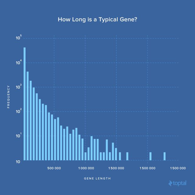
.describe() provides basic length statistics:
Mean gene length: ~36,000 bases
Median gene length: ~5,200 bases
Minimum gene length: 8 bases
Maximum gene length: ~2.3 million bases
The mean being much larger than the median suggests a right-skewed length distribution. Let’s visualize this.
1
2
3
4
5
| import matplotlib as plt
ndf.length.plot(kind='hist', bins=50, logy=True)
plt.show()
|
Pandas simplifies matplotlib integration, making DataFrame and Series plotting easy.
Here, kind='hist' requests a histogram with 50 bins and a logarithmic y-axis (logy=True).
The histogram shows that most genes fall within the first bin. However, some are over two million bases long. Let’s identify them:
1
2
3
4
5
6
7
8
9
| In [39]: ndf[ndf.length > 2e6].sort_values('length').ix[::-1]
Out[39]:
seqid source type start end score strand phase gene_name gene_id desc length
2309345 7 ensembl_havana gene 146116002 148420998 . + . CNTNAP2 ENSG00000174469 contactin associated protein-like 2 [Source:HG... 2304997
2422510 9 ensembl_havana gene 8314246 10612723 . - . PTPRD ENSG00000153707 protein tyrosine phosphatase%2C receptor type ... 2298478
2527169 X ensembl_havana gene 31097677 33339441 . - . DMD ENSG00000198947 dystrophin [Source:HGNC Symbol%3BAcc:HGNC:2928] 2241765
440886 11 ensembl_havana gene 83455012 85627922 . - . DLG2 ENSG00000150672 discs large MAGUK scaffold protein 2 [Source:H... 2172911
2323457 8 ensembl_havana gene 2935353 4994972 . - . CSMD1 ENSG00000183117 CUB and Sushi multiple domains 1 [Source:HGNC ... 2059620
1569914 20 ensembl_havana gene 13995369 16053197 . + . MACROD2 ENSG00000172264 MACRO domain containing 2 [Source:HGNC Symbol%... 2057829
|
The longest gene is CNTNAP2 (contactin-associated protein-like 2). According to its wikipedia page:
This gene spans almost 1.6% of chromosome 7 and is one of the largest in the human genome.
Our analysis confirms this! Now, let’s look at the shortest genes:
1
2
3
4
5
6
7
8
| In [40]: ndf.sort_values('length').head()
Out[40]:
seqid source type start end score strand phase gene_name gene_id desc length
682278 14 havana gene 22438547 22438554 . + . TRDD1 ENSG00000223997 T cell receptor delta diversity 1 [Source:HGNC... 8
682282 14 havana gene 22439007 22439015 . + . TRDD2 ENSG00000237235 T cell receptor delta diversity 2 [Source:HGNC... 9
2306836 7 havana gene 142786213 142786224 . + . TRBD1 ENSG00000282431 T cell receptor beta diversity 1 [Source:HGNC ... 12
682286 14 havana gene 22449113 22449125 . + . TRDD3 ENSG00000228985 T cell receptor delta diversity 3 [Source:HGNC... 13
1879625 4 havana gene 10238213 10238235 . - . AC006499.9 ENSG00000271544 23
|
The length difference between the extremes is five orders of magnitude (2.3 million vs. 8), highlighting life’s incredible diversity.
A single gene can produce multiple proteins through alternative splicing, a concept we haven’t explored here. The GFF3 file contains this information, but it’s beyond this post’s scope.
Gene Distribution Among Chromosomes
Finally, let’s analyze gene distribution across chromosomes, which also demonstrates the .merge method for combining DataFrames. Intuitively, longer chromosomes should contain more genes. Let’s see.
 1
 2
 3
 4
 5
 6
 7
 8
 9
10
11
12
13
14
15
16
17
18
19
20
21
22
23
24
25
26
27
28
29
| In [53]: ndf = ndf[ndf.seqid.isin(chrs)]
In [54]: chr_gene_counts = ndf.groupby('seqid').count().ix[:, 0].sort_values().ix[::-1]
Out[54]: chr_gene_counts
seqid
1 3902
2 2806
11 2561
19 2412
17 2280
3 2204
6 2154
12 2140
7 2106
5 2002
16 1881
X 1852
4 1751
9 1659
8 1628
10 1600
15 1476
14 1449
22 996
20 965
13 872
18 766
21 541
Y 436
Name: source, dtype: int64
|
We reuse the chrs variable to exclude unassembled sequences. The output confirms that the largest chromosome, Chromosome 1, has the most genes. While Chromosome Y has the fewest genes, it’s not the smallest chromosome.
Surprisingly, there seem to be no genes in the mitochondrion (MT). This is incorrect.
Filtering the original df DataFrame reveals that all MT genes come from the insdc source, which we excluded when creating edf (focusing on havana, ensembl, and ensembl_havana).
 1
 2
 3
 4
 5
 6
 7
 8
 9
10
11
12
13
14
15
16
17
18
| In [134]: df[(df.type == 'gene') & (df.seqid == 'MT')]
Out[134]:
seqid source type start end score strand phase attributes
2514003 MT insdc gene 648 1601 . + . ID=gene:ENSG00000211459;Name=MT-RNR1;biotype=M...
2514009 MT insdc gene 1671 3229 . + . ID=gene:ENSG00000210082;Name=MT-RNR2;biotype=M...
2514016 MT insdc gene 3307 4262 . + . ID=gene:ENSG00000198888;Name=MT-ND1;biotype=pr...
2514029 MT insdc gene 4470 5511 . + . ID=gene:ENSG00000198763;Name=MT-ND2;biotype=pr...
2514048 MT insdc gene 5904 7445 . + . ID=gene:ENSG00000198804;Name=MT-CO1;biotype=pr...
2514058 MT insdc gene 7586 8269 . + . ID=gene:ENSG00000198712;Name=MT-CO2;biotype=pr...
2514065 MT insdc gene 8366 8572 . + . ID=gene:ENSG00000228253;Name=MT-ATP8;biotype=p...
2514069 MT insdc gene 8527 9207 . + . ID=gene:ENSG00000198899;Name=MT-ATP6;biotype=p...
2514073 MT insdc gene 9207 9990 . + . ID=gene:ENSG00000198938;Name=MT-CO3;biotype=pr...
2514080 MT insdc gene 10059 10404 . + . ID=gene:ENSG00000198840;Name=MT-ND3;biotype=pr...
2514087 MT insdc gene 10470 10766 . + . ID=gene:ENSG00000212907;Name=MT-ND4L;biotype=p...
2514091 MT insdc gene 10760 12137 . + . ID=gene:ENSG00000198886;Name=MT-ND4;biotype=pr...
2514104 MT insdc gene 12337 14148 . + . ID=gene:ENSG00000198786;Name=MT-ND5;biotype=pr...
2514108 MT insdc gene 14149 14673 . - . ID=gene:ENSG00000198695;Name=MT-ND6;biotype=pr...
2514115 MT insdc gene 14747 15887 . + . ID=gene:ENSG00000198727;Name=MT-CYB;biotype=pr...
|
This snippet demonstrates combining conditions during filtering with & (logical “and”). The logical “or” operator is |.
Parentheses around each condition are mandatory, unlike in standard Python, which uses literal and and or.
Let’s use the gdf DataFrame from earlier to get each chromosome’s length:
 1
 2
 3
 4
 5
 6
 7
 8
 9
10
11
12
13
14
15
16
17
18
19
20
21
22
23
24
25
26
27
28
29
30
| In [61]: gdf = gdf[gdf.seqid.isin(chrs)]
In [62]: gdf.drop(['start', 'end', 'score', 'strand', 'phase' ,'attributes'], axis=1, inplace=True)
In [63]: gdf.sort_values('length').ix[::-1]
Out[63]:
seqid source type length
0 1 GRCh38 chromosome 248956422
1364641 2 GRCh38 chromosome 242193529
1705855 3 GRCh38 chromosome 198295559
1864567 4 GRCh38 chromosome 190214555
1964921 5 GRCh38 chromosome 181538259
2080148 6 GRCh38 chromosome 170805979
2196981 7 GRCh38 chromosome 159345973
2514125 X GRCh38 chromosome 156040895
2321361 8 GRCh38 chromosome 145138636
2416560 9 GRCh38 chromosome 138394717
328938 11 GRCh38 chromosome 135086622
235068 10 GRCh38 chromosome 133797422
483370 12 GRCh38 chromosome 133275309
634486 13 GRCh38 chromosome 114364328
674767 14 GRCh38 chromosome 107043718
767312 15 GRCh38 chromosome 101991189
865053 16 GRCh38 chromosome 90338345
990810 17 GRCh38 chromosome 83257441
1155977 18 GRCh38 chromosome 80373285
1559144 20 GRCh38 chromosome 64444167
1201561 19 GRCh38 chromosome 58617616
2594560 Y GRCh38 chromosome 54106423
1647482 22 GRCh38 chromosome 50818468
1616710 21 GRCh38 chromosome 46709983
2513999 MT GRCh38 chromosome 16569
|
We drop irrelevant columns for clarity.
.drop can remove multiple columns in one go.
The MT entry remains; we’ll address it shortly. Now, let’s merge the two datasets based on the seqid column.
 1
 2
 3
 4
 5
 6
 7
 8
 9
10
11
12
13
14
15
16
17
18
19
20
21
22
23
24
25
26
27
28
29
30
31
32
33
34
| In [73]: cdf = chr_gene_counts.to_frame(name='gene_count').reset_index()
In [75]: cdf.head(2)
Out[75]:
seqid gene_count
0 1 3902
1 2 2806
In [78]: merged = gdf.merge(cdf, on='seqid')
In [79]: merged
Out[79]:
seqid source type length gene_count
0 1 GRCh38 chromosome 248956422 3902
1 10 GRCh38 chromosome 133797422 1600
2 11 GRCh38 chromosome 135086622 2561
3 12 GRCh38 chromosome 133275309 2140
4 13 GRCh38 chromosome 114364328 872
5 14 GRCh38 chromosome 107043718 1449
6 15 GRCh38 chromosome 101991189 1476
7 16 GRCh38 chromosome 90338345 1881
8 17 GRCh38 chromosome 83257441 2280
9 18 GRCh38 chromosome 80373285 766
10 19 GRCh38 chromosome 58617616 2412
11 2 GRCh38 chromosome 242193529 2806
12 20 GRCh38 chromosome 64444167 965
13 21 GRCh38 chromosome 46709983 541
14 22 GRCh38 chromosome 50818468 996
15 3 GRCh38 chromosome 198295559 2204
16 4 GRCh38 chromosome 190214555 1751
17 5 GRCh38 chromosome 181538259 2002
18 6 GRCh38 chromosome 170805979 2154
19 7 GRCh38 chromosome 159345973 2106
20 8 GRCh38 chromosome 145138636 1628
21 9 GRCh38 chromosome 138394717 1659
22 X GRCh38 chromosome 156040895 1852
23 Y GRCh38 chromosome 54106423 436
|
As chr_gene_counts is a Series (which doesn’t support merging), we convert it to a DataFrame with .to_frame.
.reset_index() turns the original index (seqid) into a new column and resets the index to 0-based integers.
cdf.head(2) shows the result. Next, we use .merge to combine the DataFrames based on seqid.
The merged DataFrame still lacks the MT entry because .merge defaults to an inner join. You can perform left, right, or outer joins by adjusting the how parameter (see documentation for details).
You might encounter the related .join method. Both .merge and .join combine DataFrames but have different APIs.
The official documentation states:
The related DataFrame.join method, uses merge internally for the index-on-index and index-on-column(s) joins, but joins on indexes by default rather than trying to join on common columns (the default behavior for merge). If you are joining on index, you may wish to use DataFrame.join to save yourself some typing.
In essence, .merge is more general and used internally by .join.
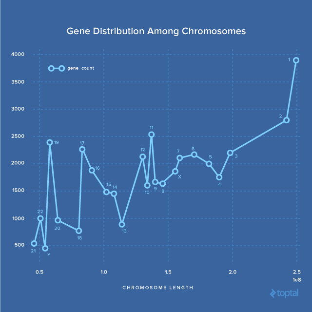
Finally, let’s calculate the correlation between chromosome length and gene_count.
1
2
3
4
5
| In [81]: merged[['length', 'gene_count']].corr()
Out[81]:
length gene_count
length 1.000000 0.728221
gene_count 0.728221 1.000000
|
.corr calculates the Pearson correlation between all column pairs in a DataFrame.
We have only one pair, and the correlation is positive (0.73).
This indicates that larger chromosomes tend to have more genes. Let’s visualize this after sorting by length:
1
2
3
4
5
6
7
8
| ax = merged[['length', 'gene_count']].sort_values('length').plot(x='length', y='gene_count', style='o-')
# add some margin to both ends of x axis
xlim = ax.get_xlim()
margin = xlim[0] * 0.1
ax.set_xlim([xlim[0] - margin, xlim[1] + margin])
# Label each point on the graph
for (s, x, y) in merged[['seqid', 'length', 'gene_count']].sort_values('length').values:
ax.text(x, y - 100, str(s))
|
While there’s a positive correlation overall, it doesn’t hold true for every chromosome. Notably, Chromosomes 17, 16, 15, 14, and 13 exhibit a negative correlation, meaning the gene count decreases as chromosome size increases.
Findings and Future Research
This concludes our exploration of manipulating a human genome annotation file (GFF3 format) using the SciPy stack, primarily employing IPython, Pandas, and matplotlib. We learned common Pandas operations and uncovered intriguing facts about our genome:
- Despite the first draft being over 15 years old, about 0.37% of the human genome remains incomplete.
- This particular GFF3 file reveals approximately 42,000 genes in the human genome.
- Gene lengths vary drastically, from a few dozen to over two million bases.
- Gene distribution across chromosomes is uneven. Generally, larger chromosomes harbor more genes, but some show an inverse correlation.
The GFF3 file is rich in information, and we’ve only scratched the surface. Further exploration could involve these questions:
- How many transcripts does a gene typically have? What proportion of genes have multiple transcripts?
- What is the typical number of isoforms per transcript?
- How many exons, CDS, and UTRs does a transcript typically have? What are their size distributions?
- Can we categorize genes based on their function described in the description column?