Adversarial Machine Learning: Strategies for Attacking and Defending ML Models

Today, machine learning models are used in many real-world computer vision applications, including self-driving cars, facial recognition, cancer detection, and even in cutting-edge stores to track customer purchases and charge their credit cards as they exit.

The remarkable accuracy of these machine learning systems has spurred a surge in their application. While the underlying mathematics have been understood for decades, the recent emergence of powerful GPUs has provided the computational power needed to develop and experiment with sophisticated machine learning systems. Today’s state-of-the-art computer vision models rely on deep neural networks with millions of parameters and hardware that was unimaginable a decade ago.

In 2012, Alex Krizhevsky et al. pioneered the implementation of a deep convolutional network, establishing a new benchmark in object classification. Since then, numerous refinements to their model have been published (VGG, ResNet, Inception, etc.), each improving accuracy. Recently, machine learning models have reached and even surpassed human-level accuracy in many computer vision tasks.

While incorrect predictions from machine learning models were once common, they are now rare. We have come to expect flawless performance, especially in real-world deployments.

Machine learning models were typically trained and evaluated in controlled environments like competitions and academic research. However, as these models are increasingly deployed in real-world settings, security vulnerabilities arising from model errors have emerged as a serious concern.

This article aims to demonstrate how state-of-the-art deep neural networks used in image recognition can be easily manipulated to produce incorrect predictions. We will explore common attack strategies and then discuss how to defend our models against them.

Adversarial Machine Learning Examples

Let’s start with a simple question: What are adversarial machine learning examples?

Adversarial examples are carefully crafted inputs designed to mislead a machine learning model.

For the purpose of this article, we will focus on image classification models. Therefore, adversarial examples will be images manipulated by an attacker to cause misclassification.

Consider a GoogLeNet trained on ImageNet for image classification as our machine learning model. Below are two images of a panda that are visually indistinguishable to humans. The left image is a clean image from the ImageNet dataset used to train the GoogLeNet model. The right image is subtly altered by adding the noise vector shown in the center. The model correctly classifies the first image as a panda. However, it confidently misclassifies the second image as a gibbon.

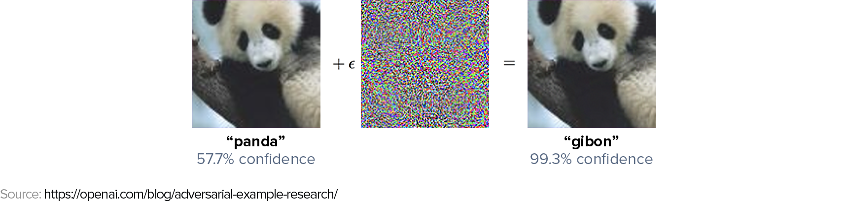
Two side-by-side images of a panda. The second image looks identical to the first, but is labeled as a different animal. A third image of what appears to be random static is between them, demonstrating the layer that was added to the second panda image to confound the model.

It’s important to note that the noise added to the original image is not random; it’s the result of a deliberate optimization process by the attacker.

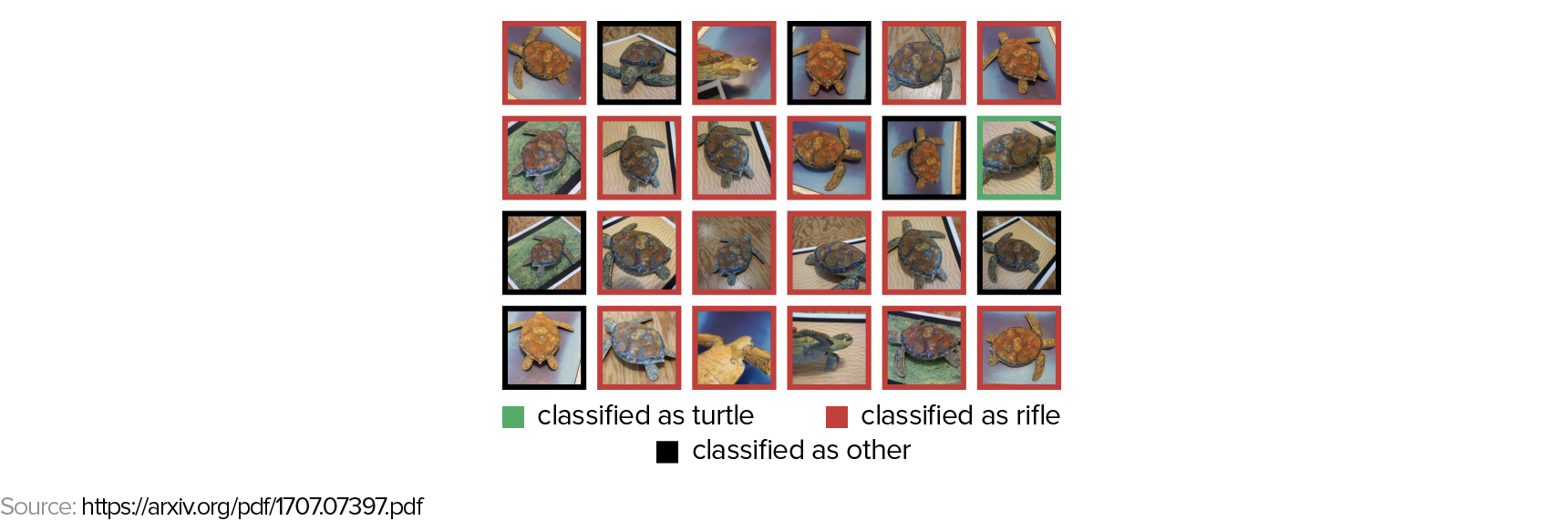
Another example involves the creation of 3D adversarial examples using a 3D printer. The image below displays various perspectives of a 3D-printed turtle and the misclassifications made by the Google Inception v3 model.

An image showing a grid of turtle images, some of which are classified correctly as turtles, some of which are classified as rifles, and a few of which are classified as other

How can highly accurate, even superhuman, models make such seemingly obvious errors?

Before examining the vulnerabilities of neural network models, let’s remember that humans have their own set of adversarial examples. Observe the following image. What do you perceive? A spiral or a series of concentric circles?

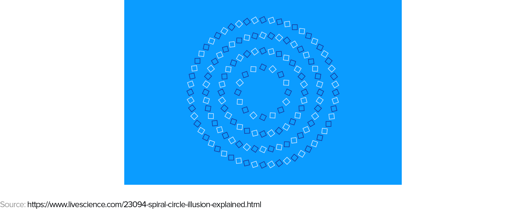
These examples highlight that machine learning models and human vision must rely on significantly different internal representations when interpreting images.

In the next section, we will explore methods for generating adversarial examples.

How to Generate Adversarial Examples

Let’s start with a simple question: What constitutes an adversarial example?

Adversarial examples are created by taking a correctly classified image and introducing a small perturbation that leads to misclassification by the ML model.

Assume an attacker possesses complete knowledge of the target model. This means they can calculate the model’s loss function $J(\theta, X, y)$, where $X$ is the input image, $y$ is the output class, and $\theta$ represents the model’s internal parameters. For classification tasks, this loss function is usually the negative log-likelihood.

In this white-box scenario, several attack strategies exist, each balancing computational cost and success rate. These methods generally aim to maximize the change in the model’s loss function while minimizing the perturbation to the input image. The higher the dimensionality of the input image space, the easier it becomes to generate adversarial examples that are imperceptible to humans.

L-BFGS Method

Adversarial examples ${x}’$ are found by solving the following box-constrained optimization problem:

$ \begin{matrix} \text{minimize } c \cdot \left \| x - {x}' \right \|^2_2 + \text{loss}_{f,1} {x}' \\ \text{such that } {x}' \epsilon \left [0, 1 \right ]^n \end{matrix} $

Here, $c > 0$ is a parameter that also needs to be determined. In essence, we seek adversarial images ${x}’$ where the weighted sum of the distortion from the clean image ($\left | x - {x}’ \right |$) and the loss with respect to the incorrect class is minimized.

For complex models like deep neural networks, this optimization problem lacks a closed-form solution, requiring iterative numerical methods. Consequently, this L-BFGS method is slow, but it boasts a high success rate.

Fast Gradient Sign (FGS)

The fast gradient sign (FGS) method linearly approximates the loss function around the initial point defined by the clean image vector $X$ and the true class $y$.

This approximation assumes that the gradient of the loss function points towards the direction of maximal loss change for the input vector. To limit perturbation size, only the sign of the gradient is used, not its magnitude, and it is scaled by a small factor epsilon.

This ensures that the pixel-wise difference between the original and modified images remains smaller than epsilon (measured by the L_infinity norm).

$ X^{adv} = X + \epsilon \text{ sign} \left( \bigtriangledown_x J \left( X, y_{true} \right) \right) $

The gradient can be efficiently computed using backpropagation, making this method one of the fastest and computationally cheapest to implement. However, it has a lower success rate than more computationally expensive methods like L-BFGS.

The authors of Adversarial Machine Learning at Scale reported a success rate between 63% and 69% for top-1 prediction on the ImageNet dataset, with epsilon values between 2 and 32. For linear models like logistic regression, the fast gradient sign method is precise. In these cases, the authors of another research paper on adversarial examples report a 99% success rate.

Iterative Fast Gradient Sign

A straightforward extension of the previous method involves applying the fast gradient sign method multiple times with a smaller step size alpha. The total step length is then clipped to guarantee that the distortion between the clean and adversarial images remains below epsilon.

$ X^{adv}_0 = X, X^{adv}_{N + 1} = Clip_{X, \epsilon} \left\{ X^{adv}_{N} + \alpha \text{ sign} \left( \bigtriangledown_X J \left( X^{adv}_N, y_{true} \right) \right) \right\} $

Other techniques, such as those proposed in Nicholas Carlini’s paper, improve upon the L-BFGS method. While computationally expensive, they achieve higher success rates.

However, in many real-world situations, attackers lack complete knowledge of the target model’s loss function. In these cases, they must resort to black-box strategies.

Black-box Attack

Research has consistently shown that adversarial examples exhibit good transferability between models. This means an example designed for one model (A) can often effectively target another model trained on similar data.

Attackers can exploit this transferability property when they lack complete information about the target model. Here’s how:

Query the target model with inputs $X_i$ for $i=1…n$ and record the outputs $y_i$.
Use the collected training data $(X_i, y_i)$ to build a substitute model.
Apply any of the aforementioned white-box algorithms to generate adversarial examples for the substitute model. Many of these examples will successfully transfer and effectively target the original model.

A successful implementation of this strategy against a commercial machine learning model is detailed in this Computer Vision Foundation paper.

Defenses Against Adversarial Examples

Attackers exploit all available information about a model when crafting their attacks. Therefore, limiting the information revealed by the model at prediction time makes it harder to create successful attacks.

A simple but effective first line of defense is to avoid displaying confidence scores for each predicted class in production environments. Instead, the model should only output the top $N$ (e.g., 5) most likely classes. Providing confidence scores to end-users allows attackers to numerically estimate the gradient of the loss function, enabling white-box attacks like the fast gradient sign method. The Computer Vision Foundation paper mentioned earlier demonstrates this technique against a commercial machine learning model.

Let’s examine two defenses proposed in the literature.

Defensive Distillation

This method aims to create a new model with significantly smaller gradients than the original, undefended model. When gradients are small, techniques like FGS or Iterative FGS become ineffective because attackers require much larger input image distortions to significantly alter the loss function.

Defensive distillation introduces a new parameter $T$, called temperature, to the last softmax layer of the network:

$ \text{softmax} \left( x, T \right)_i = \frac{e^{x_i/T}}{\Sigma_j e^{x_j/T}} $

Note that a $T$ value of 1 results in the standard softmax function. Higher $T$ values lead to smaller gradients of the loss with respect to the input images.

Defensive distillation follows these steps:

Train a teacher network with a high temperature $T » 1$.
Use the trained teacher network to generate soft-labels for each image in the training set. A soft-label represents the model’s assigned probabilities for each class. For example, for a parrot image, the teacher model might output soft labels like (90% parrot, 10% macaw).
Train a second network, the distilled network, on the soft-labels, again using the high temperature $T$. Training with soft-labels mitigates overfitting and improves the distilled network’s out-of-sample accuracy.
Finally, at prediction time, run the distilled network with a temperature $T=1$.

Defensive distillation effectively protects against the attacks described in Distillation as a Defense to Adversarial Perturbations against Deep Neural Networks.

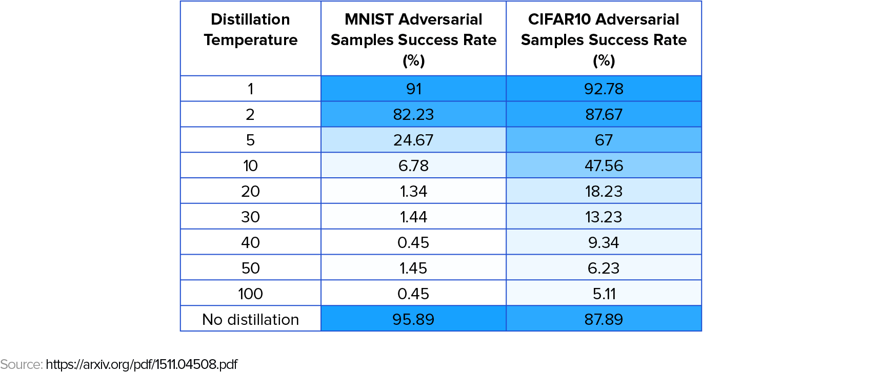
Image of a table showing the success rate based on distillation temperature. Generally, the higher the temperature, the lower the success rate, for both MNIST and CIFAR10 adversarial samples.

However, a later paper by University of California, Berkeley reserachers introduced new attack methods that circumvent defensive distillation, demonstrating that it is not a universal solution against adversarial examples. These attacks are enhancements of the L-BFGS method.

Adversarial Training

Currently, adversarial training is the most effective defense strategy. This involves generating adversarial examples and incorporating them into the model’s training data. The idea is that by exposing the model to adversarial examples during training, its performance against similar examples at prediction time improves.

Ideally, all known attack methods would be used to generate adversarial examples for training. However, for large, high-dimensional datasets like ImageNet, robust attack methods like L-BFGS and the improvements described in the Berkeley paper are computationally prohibitive. In practice, faster methods like FGS or iterative FGS are used.

Adversarial training employs a modified loss function that combines the usual loss function for clean examples with a loss function for adversarial examples.

$ Loss = \frac{1}{\left( m - k \right)} \left( \sum_{i \epsilon CLEAN} {L \left( X_i | y_i \right) + \lambda} \sum_{i \epsilon ADV} {L \left( X*{adv}_i | y_i \right)} \right) $

During training, for each batch of $m$ clean images, $k$ adversarial images are generated using the current network state. Both clean and adversarial examples are fed through the network, and the combined loss is calculated using the formula above.

Ensemble adversarial training, an improvement presented in this conference paper, utilizes multiple pre-trained models to generate adversarial examples instead of relying on the current network. This approach enhances the network’s robustness against black-box attacks on ImageNet. It emerged as the winner of the first round of the NIPS 2017 competition on Defenses against Adversarial Attacks.

Conclusions and Further Steps

Attacking machine learning models remains easier than defending them. Without adequate defense strategies, state-of-the-art models deployed in real-world applications are susceptible to adversarial examples, potentially leading to critical security breaches. Adversarial training, where adversarial examples are generated and included in the training data alongside clean examples, is currently the most effective defense.

To evaluate the robustness of your image classification models against different attacks, consider using the open-source Python library cleverhans. It allows testing various attack methods, including those discussed here, against your models. You can also use it to perform adversarial training and enhance your model’s resilience to adversarial examples.

The search for new attack and defense strategies is an active area of research. Both theoretical and empirical advancements are needed to ensure the robustness and security of machine learning models in real-world applications.

I encourage readers to explore these techniques and contribute to the growing body of knowledge. I welcome any feedback on this article.